PostgreSQL statistical analysis using PL / R
Friends, at last year’s PG Day'15 Russia conference, one of our speakers, Joseph Conway, presented interesting material on the use of the PL / R extension that he created and has supported for over ten years, which allows you to use the language for statistical analysis of R inside your favorite Database. I want to bring to your attention a follow-up article created on the basis of the materials presented in the Joe report . The purpose of this publication is to acquaint you with the possibilities of the PL / R language. I hope you find the information presented here useful to you.

Recent Big Data trends have encouraged the convergence of analytics and data, while PL / R has been unobtrusively providing such a service for 12 years now! If suddenly you are not in the know, PL / R is an extension for PostgreSQL that allows you to use R, the language for mathematical calculations, directly from PostgreSQL in order to easily and easily get detailed analytics. The extension is available and has been actively improved since 2003. It works with all supported versions of PostgreSQL and all recent versions of R. Thousands of people around the world have already appreciated its convenience and effectiveness. Let’s take a look at what PL / R is, discuss the advantages and disadvantages of this approach to data analysis, and consider a few examples for illustrative purposes.
To begin, let us define basic concepts. R is a programming language for statistical data processing and graphics, as well as a free open source software environment. And PostgreSQL is a powerful free object-relational database management system that has been actively developed for over 25 years and has earned an excellent reputation due to its reliability, as well as correctness and integrity of data. And finally, PL / R. As mentioned above, this is a procedural R language handler for PostgreSQL, which allows you to write SQL functions in R.
So what are the benefits of PL / R? Firstly, PL / R contributes to the development of human knowledge and skills, since mathematics, statistics, databases and the web are different specializations, but all of them will have to be mastered to one degree or another to work with PL / R. Secondly, this extension stimulates the improvement of hardware, because you need a server that can withstand the analysis of large data sets. Thirdly, processing efficiency will increase, since you no longer have to transfer large data sets across the entire network, and throughput will increase. Fourth, you can be sure that the analysis will be carried out sequentially. Fifth, PL / R makes a system of any complexity understandable and maintainable. And finally, with rich functionality and a huge ecosystem, PL / R expands R.
But, of course, there are also disadvantages. A PostgreSQL user will likely find that PL / R is slower, especially on simple tasks. And for the R programmer, the debugging process will become more complicated and the analysis will become less flexible. In addition, both will have to learn a new language.
This is what the standard function in R looks like:
Creating functions in PL / R is slightly different, but similar to other PLs in PostgreSQL:
Here is an example:
It is difficult to list everything that can be done with PL / R, but let's dwell on some important properties, such as:
Thanks to compatibility with PostgreSQL, we can prototype using R, and then move to PL / R to execute in “production”. Also a definite plus is that all queries are executed in the current database. Driver and connection settings are ignored, so dbDriver, dbConnect, dbDisconnect and dbUnloadDriver do not require additional effort:
Let's give a couple of examples for illustrative purposes. Suppose we need to turn to PostgreSQL from R to solve the famous traveling salesman problem, which we will discuss in detail later:
And here is the same function in PL / R:
Here is what R ultimately outputs to us:
And the same function in PL / R:
As you can see, the result is the same.
Now let's talk about the units (aggregates). One of the most useful features of PostgreSQL is the ability to write its own aggregate functions. Aggregates in PostgreSQL can be expanded using SQL commands. In this case, the state transition function and, sometimes, the final function are indicated. The initial condition of the transition function can also be specified. And you can enjoy these benefits when working with PL / R.
Here is an example of a PL / R function that implements a new aggregate. Until recently, this was not possible to do from PostgreSQL, GROUPING SETS functionality appeared only in version 9.5, while PL / R allows you to do this in any version of PG. I will create an aggregate function based on the real data of one production company and call it quartile:
R allows you to display data in the form of nice graphs. In this case, the box diagram was used:

According to the graph, it is clear that one of the production stations is less productive than the others, and measures must be taken to fix this.
Separately, it is worth stopping at window functions . They have been available in PostgreSQL since version 8.4, and are great for statistical analysis. Window functions are similar to aggregate ones, but, unlike them, they do not group strings, but allow calculations in sets of strings associated with the current row, having access not only to the current row of the query result. In other words, your data is divided into sections, and there is a window that slides through these sections and produces the result for each data group:
Few procedural languages PostgreSQL support window functions, but in PL / R they are very useful. Here's an example: create a random data table that simulates earnings and stock prices.
And we will write a function in order to find out whether it is possible to predict revenues this year, based on the indicators of last year, using the simple regression method.
As you can see, the function calculated the dependence of income on the indicators of previous years.
The last thing worth discussing in detail is the mechanisms for returning R objects and their storage methods.
We give an example with stock data. To do this, take the Hi-Low-Close data from Yahoo for any stock ticker. Let's build a chart with Bollinger lines and volume. We need additional R packets, which can be obtained from R with the following command:
Now make a request:
A typical server will require a screen buffer to create a graph:
Now call the function from PHP for the CYMI ticker:
And here we get such a schedule:
Agree, it is surprising that we can write a dozen lines in PL / R and less than a dozen lines in PHP, and in the end get such a detailed visual display and analysis of our data.
To consolidate the information, consider more complex examples. I think many people are familiar with Benford's law, or the law of the first digit, which describes the probability of a certain first significant digit appearing in the distributions of quantities taken from real life. But some are unaware of its existence and themselves distribute the data as they need, instead of applying the law.
Benford's law can be used to identify potential fraud: with its help, you can build an approximate geometric sequence based on several initial values, and then compare it with real data and find inconsistencies. This method can be applied to sales schedules, census data, cost reports, etc.
Consider the example of the California Energy Optimization Program. To begin, create and fill out a table with data on investment in the project (data is available at http://open-emv.com/data ):
Now we write the function of Benford's law:
And run the comparison:
It seems that the real data is in line with the forecast, so there are no signs of fraud in this case.
Let's get back to the traveling salesman problem. This is one of the most famous problems of combinatorial optimization, which consists in finding the most profitable route that passes through these cities at least once, and then returns to the original city. In the conditions of the problem, criteria for the profitability of the route (the shortest, cheapest, cumulative criterion, and so on) and the corresponding matrix of distances, cost, and the like are indicated. As a rule, it is indicated that the route should go through each city only once. Let's look at this particular option.
First, create and populate a table with all the cities that you need to visit:
To get the result, I have to write a couple of auxiliary queries. The first will create the route that I want to get on the output:
And the second is the data that I enter in plr_modules, and the type of the resulting data:
Create the main PL / R function:
Now we need to set the make.route () function:
And the make.map () function:
We start the function of receiving TSP tags:
Advanced view:
Thus, we got the order in which it is worth visiting these cities, the distance between them, etc. In addition, we also have a visual solution to the traveling salesman problem:

Consider another example, this time with seismic data.
When an earthquake occurs, it usually lasts 15-20 seconds, and seismologists collect data on the intensity of its vibrations. That is, we have time series (timeseries) of data in the format of a waveform (waveform data). The data is stored as an array of floating point numbers (floats) recorded during a seismic event with a constant sampling frequency. They are available from online sources in separate files for each activity. Each file contains about 16,000 elements.
We load 1000 seismic activities using PL / pgSQL:
This can be done in another way, with the help of R, and it will take half the time - that is the rare case when using PL / R speeds up rather than slows down the process:
Let's create an oscillogram:
We get this picture for a specific earthquake:

Now we need to analyze it, for example, to find out how best to design buildings in an area with similar seismic activity. You probably remember from the school physics course such a thing as “resonant frequency”. Just in case, let me remind you that this is such an oscillation frequency at which the oscillation amplitude increases sharply. This frequency is determined by the properties of the system. That is, in a zone with seismic activity, it is necessary to design the structures so that their resonant frequency does not coincide with the frequency of earthquakes. This can be done using R:
And this is how the final result looks, showing the frequency of vibrations and their amplitude:

Having such a schedule before his eyes, the architect can make calculations and design a structure that will not collapse at the first tremor.
As you can see, PL / R has many areas of application, as it allows you to connect advanced analytics with databases and at the same time use the functionality of R and PostgreSQL with all their advantages. I hope this article will be useful to you, and you will find application for such an effective and multifunctional tool.
We also invite you to familiarize yourself with the source materials on the basis of which this article was prepared: presentation and videofrom a performance by Joe Conway at PG Day'15 Russia. If the topic of using PL / R seems interesting to you, be sure to share your thoughts and ideas. Who knows, maybe we will organize a report on this topic at the upcoming PG Day'16 in July. As usual, we are waiting for your comments.
Recent Big Data trends have encouraged the convergence of analytics and data, while PL / R has been unobtrusively providing such a service for 12 years now! If suddenly you are not in the know, PL / R is an extension for PostgreSQL that allows you to use R, the language for mathematical calculations, directly from PostgreSQL in order to easily and easily get detailed analytics. The extension is available and has been actively improved since 2003. It works with all supported versions of PostgreSQL and all recent versions of R. Thousands of people around the world have already appreciated its convenience and effectiveness. Let’s take a look at what PL / R is, discuss the advantages and disadvantages of this approach to data analysis, and consider a few examples for illustrative purposes.
To begin, let us define basic concepts. R is a programming language for statistical data processing and graphics, as well as a free open source software environment. And PostgreSQL is a powerful free object-relational database management system that has been actively developed for over 25 years and has earned an excellent reputation due to its reliability, as well as correctness and integrity of data. And finally, PL / R. As mentioned above, this is a procedural R language handler for PostgreSQL, which allows you to write SQL functions in R.
So what are the benefits of PL / R? Firstly, PL / R contributes to the development of human knowledge and skills, since mathematics, statistics, databases and the web are different specializations, but all of them will have to be mastered to one degree or another to work with PL / R. Secondly, this extension stimulates the improvement of hardware, because you need a server that can withstand the analysis of large data sets. Thirdly, processing efficiency will increase, since you no longer have to transfer large data sets across the entire network, and throughput will increase. Fourth, you can be sure that the analysis will be carried out sequentially. Fifth, PL / R makes a system of any complexity understandable and maintainable. And finally, with rich functionality and a huge ecosystem, PL / R expands R.
But, of course, there are also disadvantages. A PostgreSQL user will likely find that PL / R is slower, especially on simple tasks. And for the R programmer, the debugging process will become more complicated and the analysis will become less flexible. In addition, both will have to learn a new language.
This is what the standard function in R looks like:
func_name <- function(myarg1 [,myarg2...]) {
    function body referencing myarg1 [, myarg2 ...]
}
Creating functions in PL / R is slightly different, but similar to other PLs in PostgreSQL:
CREATE OR REPLACE FUNCTION func_name(arg-type1 [, arg-type2 ...])
    RETURNS return-type AS $$
    function body referencing arg1 [, arg2 ...]
$$ LANGUAGE 'plr';
CREATE OR REPLACE FUNCTION func_name(myarg1 arg-type1 [, myarg2 arg-type2 ...])
    RETURNS return-type AS $$
    function body referencing myarg1 [, myarg2 ...]
$$ LANGUAGE 'plr';
Here is an example:
CREATE EXTENSION plr;
CREATE OR REPLACE FUNCTION test_dtup(OUT f1 text, OUT f2 int)
RETURNS SETOF record AS $$
    data.frame(letters[1:3],1:3)
$$ LANGUAGE 'plr';
SELECT * FROM test_dtup();
f1 | f2
----+----
a | 1
b | 2
c | 3
(3 rows)
It is difficult to list everything that can be done with PL / R, but let's dwell on some important properties, such as:
- PostgreSQL compatibility
- custom SQL aggregates;
- window functions;
- translate an R object into bytea (binary strings).
Thanks to compatibility with PostgreSQL, we can prototype using R, and then move to PL / R to execute in “production”. Also a definite plus is that all queries are executed in the current database. Driver and connection settings are ignored, so dbDriver, dbConnect, dbDisconnect and dbUnloadDriver do not require additional effort:
dbDriver(character dvr_name)
dbConnect(DBIDriver drv, character user, character password, character host, character dbname, character port, character tty, character options)
dbSendQuery(DBIConnection conn, character sql)
fetch(DBIResult rs, integer num_rows)
dbClearResult (DBIResult rs)
dbGetQuery(DBIConnection conn, character sql)
dbReadTable(DBIConnection conn, character name)
dbDisconnect(DBIConnection conn)
dbUnloadDriver(DBIDriver drv)
Let's give a couple of examples for illustrative purposes. Suppose we need to turn to PostgreSQL from R to solve the famous traveling salesman problem, which we will discuss in detail later:
tsp_tour_length<-function() {
    require(TSP)
    require(fields)
    require(RPostgreSQL)
    drv <- dbDriver("PostgreSQL")
    conn <- dbConnect(drv, user="postgres", dbname="plr", host="localhost")
    sql.str <- "select id, st_x(location) as x, st_y(location) as y, location from stands"
    waypts <- dbGetQuery(conn, sql.str)
    dist.matrix <- rdist.earth(waypts[,2:3], R=3949.0)
    rtsp <- TSP(dist.matrix)
    soln <- solve_TSP(rtsp)
    dbDisconnect(conn)
    dbUnloadDriver(drv)
    return(attributes(soln)$tour_length)
}
And here is the same function in PL / R:
CREATE OR REPLACE FUNCTION tsp_tour_length()
RETURNS float8 AS $$
    require(TSP)
    require(fields)
    require(RPostgreSQL)
    drv <- dbDriver("PostgreSQL")
    conn <- dbConnect(drv, user="postgres", dbname="plr", host="localhost")
    sql.str <- "select id, st_x(location) as x, st_y(location) as y, location from stands"
    waypts <- dbGetQuery(conn, sql.str)
    dist.matrix <- rdist.earth(waypts[,2:3], R=3949.0)
    rtsp <- TSP(dist.matrix)
    soln <- solve_TSP(rtsp)
    dbDisconnect(conn)
    dbUnloadDriver(drv)
    return(attributes(soln)$tour_length)
$$ LANGUAGE 'plr' STRICT;
Here is what R ultimately outputs to us:
tsp_tour_length()
[1] 2804.581
And the same function in PL / R:
SELECT tsp_tour_length();
tsp_tour_length
------------------
2804.58129355858
(1 row)
As you can see, the result is the same.
Now let's talk about the units (aggregates). One of the most useful features of PostgreSQL is the ability to write its own aggregate functions. Aggregates in PostgreSQL can be expanded using SQL commands. In this case, the state transition function and, sometimes, the final function are indicated. The initial condition of the transition function can also be specified. And you can enjoy these benefits when working with PL / R.
Here is an example of a PL / R function that implements a new aggregate. Until recently, this was not possible to do from PostgreSQL, GROUPING SETS functionality appeared only in version 9.5, while PL / R allows you to do this in any version of PG. I will create an aggregate function based on the real data of one production company and call it quartile:
CREATE OR REPLACE FUNCTION r_quartile(ANYARRAY)
RETURNS ANYARRAY AS $$
    quantile(arg1, probs = seq(0, 1, 0.25), names = FALSE)
$$ LANGUAGE 'plr';
CREATE AGGREGATE quartile (ANYELEMENT) (
    sfunc = array_append,
    stype = ANYARRAY,
    finalfunc = r_quantile,
    initcond = '{}'
);
SELECT workstation, quartile(id_val)
    FROM sample_numeric_data
    WHERE ia_id = 'G121XB8A' GROUP BY workstation;
workstation | quantile
-------------+---------------------------------
1055 | {4.19,5.02,5.21,5.5,6.89}
1051 | {3.89,4.66,4.825,5.2675,5.47}
1068 | {4.33,5.2625,5.455,5.5275,6.01}
1070 | {4.51,5.1975,5.485,5.7575,6.41}
(4 rows)
R allows you to display data in the form of nice graphs. In this case, the box diagram was used:
According to the graph, it is clear that one of the production stations is less productive than the others, and measures must be taken to fix this.
Separately, it is worth stopping at window functions . They have been available in PostgreSQL since version 8.4, and are great for statistical analysis. Window functions are similar to aggregate ones, but, unlike them, they do not group strings, but allow calculations in sets of strings associated with the current row, having access not only to the current row of the query result. In other words, your data is divided into sections, and there is a window that slides through these sections and produces the result for each data group:
Few procedural languages PostgreSQL support window functions, but in PL / R they are very useful. Here's an example: create a random data table that simulates earnings and stock prices.
CREATE TABLE test_data (
    fyear integer,
    firm float8,
    eps float8
);
INSERT INTO test_data
SELECT (b.f + 1) % 10 + 2000 AS fyear,
       floor((b.f+1)/10) + 50 AS firm,
       f::float8/100 + random()/10 AS eps
    FROM generate_series(-500,499,1) b(f);
CREATE OR REPLACE FUNCTION r_regr_slope(float8, float8)
RETURNS float8 AS
$BODY$
    slope <- NA
    y <- farg1
    x <- farg2
    if (fnumrows==9) try (slope <- lm(y ~ x)$coefficients[2])
    return(slope)
$BODY$ LANGUAGE plr WINDOW;
And we will write a function in order to find out whether it is possible to predict revenues this year, based on the indicators of last year, using the simple regression method.
SELECT *, r_regr_slope(eps, lag_eps) OVER w AS slope_R
    FROM (
        SELECT firm AS f,
               fyear AS fyr,
               eps,
               lag(eps) OVER (PARTITION BY firm ORDER BY firm, fyear) AS lag_eps
            FROM test_data
    ) AS a
    WHERE eps IS NOT NULL
    WINDOW w AS (PARTITION BY firm ORDER BY firm, fyear ROWS 8 PRECEDING);
f | fyr | eps | lag_eps | slope_r
---+------+-------------------+-------------------+-------------------
1 | 1991 | -4.99563754182309 | |
1 | 1992 | -4.96425441872329 | -4.99563754182309 |
1 | 1993 | -4.96906093481928 | -4.96425441872329 |
1 | 1994 | -4.92376988714561 | -4.96906093481928 |
1 | 1995 | -4.95884547665715 | -4.92376988714561 |
1 | 1996 | -4.93236254784279 | -4.95884547665715 |
1 | 1997 | -4.90775520844385 | -4.93236254784279 |
1 | 1998 | -4.92082695348188 | -4.90775520844385 |
1 | 1999 | -4.84991340579465 | -4.92082695348188 | 0.691850614092383
1 | 2000 | -4.86000917562284 | -4.84991340579465 | 0.700526929134053
As you can see, the function calculated the dependence of income on the indicators of previous years.
The last thing worth discussing in detail is the mechanisms for returning R objects and their storage methods.
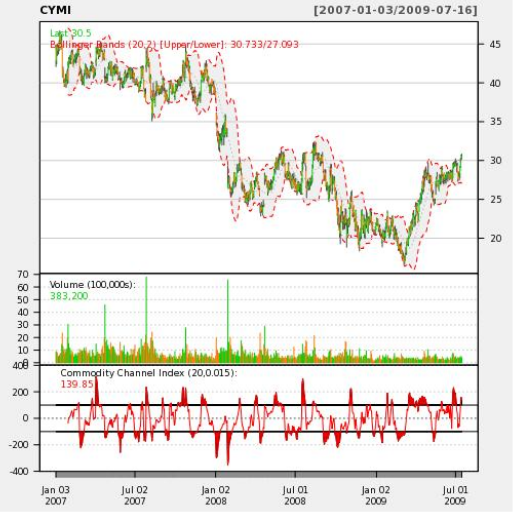
We give an example with stock data. To do this, take the Hi-Low-Close data from Yahoo for any stock ticker. Let's build a chart with Bollinger lines and volume. We need additional R packets, which can be obtained from R with the following command:
install.packages(c('xts','Defaults','quantmod','cairoDevice','RGtk2'))
Now make a request:
CREATE OR REPLACE FUNCTION plot_stock_data(sym text)
  RETURNS bytea AS
$$
    library(quantmod)
    library(cairoDevice)
    library(RGtk2)
    pixmap <- gdkPixmapNew(w=500, h=500, depth=24)
    asCairoDevice(pixmap)
    getSymbols(c(sym))
    chartSeries(get(sym), name=sym, theme="white", TA="addVo();addBBands();addCCI()")
    plot_pixbuf <- gdkPixbufGetFromDrawable(NULL, pixmap,
    pixmap$getColormap(),0, 0, 0, 0, 500, 500)
    buffer <- gdkPixbufSaveToBufferv(plot_pixbuf, "jpeg", character(0), character(0))$buffer
    return(buffer)
$$ LANGUAGE plr;
A typical server will require a screen buffer to create a graph:
Xvfb :1 -screen 0 1024x768x24
export DISPLAY=:1.0
Now call the function from PHP for the CYMI ticker:
And here we get such a schedule:
Agree, it is surprising that we can write a dozen lines in PL / R and less than a dozen lines in PHP, and in the end get such a detailed visual display and analysis of our data.
To consolidate the information, consider more complex examples. I think many people are familiar with Benford's law, or the law of the first digit, which describes the probability of a certain first significant digit appearing in the distributions of quantities taken from real life. But some are unaware of its existence and themselves distribute the data as they need, instead of applying the law.
Benford's law can be used to identify potential fraud: with its help, you can build an approximate geometric sequence based on several initial values, and then compare it with real data and find inconsistencies. This method can be applied to sales schedules, census data, cost reports, etc.
Consider the example of the California Energy Optimization Program. To begin, create and fill out a table with data on investment in the project (data is available at http://open-emv.com/data ):
CREATE TABLE open_emv_cost(value float8, district int);
COPY open_emv_cost FROM 'open-emv.cost.csv' WITH delimiter ',';
Now we write the function of Benford's law:
CREATE TYPE benford_t AS (
    actual_mean float8,
    n int,
    expected_mean float8,
    distorion float8,
    z float8
);
CREATE OR REPLACE FUNCTION benford(numarr float8[])
RETURNS benford_t AS
$$
    xcoll <- function(x) {
        return ((10 * x) / (10 ^ (trunc(log10(x)))))
    }
    numarr <- numarr[numarr >= 10]
    numarr <- xcoll(numarr)
    actual_mean <- mean(numarr)
    n <- length(numarr)
    expected_mean <- (90 / (n * (10 ^ (1/n) - 1)))
    distorion <- ((actual_mean - expected_mean) / expected_mean)
    z <- (distorion / sd(numarr))
    retval <- data.frame(actual_mean,n,expected_mean,distorion,z)
    return(retval)
$$ LANGUAGE plr;
And run the comparison:
SELECT * FROM benford(array(SELECT value FROM open_emv_cost));
-[ RECORD 1 ]-+----------------------
actual_mean | 38.1936561918275
n | 240
expected_mean | 38.8993031865999
distorion | -0.0181403505195804
z | -0.000984036908080443
It seems that the real data is in line with the forecast, so there are no signs of fraud in this case.
Let's get back to the traveling salesman problem. This is one of the most famous problems of combinatorial optimization, which consists in finding the most profitable route that passes through these cities at least once, and then returns to the original city. In the conditions of the problem, criteria for the profitability of the route (the shortest, cheapest, cumulative criterion, and so on) and the corresponding matrix of distances, cost, and the like are indicated. As a rule, it is indicated that the route should go through each city only once. Let's look at this particular option.
First, create and populate a table with all the cities that you need to visit:
CREATE TABLE stands (
    id serial primary key,
    strata integer not null,
    initage integer
);
SELECT AddGeometryColumn('','stands','boundary','4326','MULTIPOLYGON',2);
CREATE INDEX "stands_boundary_gist" ON "stands" USING gist ("boundary" gist_geometry_ops);
SELECT AddGeometryColumn('','stands','location','4326','POINT',2);
CREATE INDEX "stands_location_gist" ON "stands" USING gist ("location" gist_geometry_ops);
INSERT INTO stands (id,strata,initage,boundary,location)
    VALUES
    (
        1,1,1,
        GeometryFromText(
            'MULTIPOLYGON(((59.250000 65.000000,55.000000 65.000000,55.000000 51.750000,
            60.735294 53.470588, 62.875000 57.750000, 59.250000 65.000000 )))', 4326
        ),
        GeometryFromText('POINT( 61.000000 59.000000 )', 4326)
    ), (
        2,2,1,
        GeometryFromText(
            'MULTIPOLYGON(((67.000000 65.000000,59.250000 65.000000,62.875000 57.750000,
            67.000000 60.500000, 67.000000 65.000000 )))', 4326
        ),
        GeometryFromText('POINT( 63.000000 60.000000 )', 4326 )
    ), (
        3,3,1,
        GeometryFromText(
            'MULTIPOLYGON(((67.045455 52.681818,60.735294 53.470588,55.000000 51.750000,
            55.000000 45.000000, 65.125000 45.000000, 67.045455 52.681818 )))', 4326
        ),
        GeometryFromText('POINT( 64.000000 49.000000 )', 4326 )
    )
;
To get the result, I have to write a couple of auxiliary queries. The first will create the route that I want to get on the output:
INSERT INTO stands (id,strata,initage,boundary,location)
    VALUES
    (
        4,4,1,
        GeometryFromText(
            'MULTIPOLYGON(((71.500000 53.500000,70.357143 53.785714,67.045455 52.681818,
            65.125000 45.000000, 71.500000 45.000000, 71.500000 53.500000 )))', 4326
        ),
        GeometryFromText('POINT( 68.000000 48.000000 )', 4326)
    ), (
        5,5,1,
        GeometryFromText(
            'MULTIPOLYGON(((69.750000 65.000000,67.000000 65.000000,67.000000 60.500000,
            70.357143 53.785714, 71.500000 53.500000, 74.928571 54.642857, 69.750000 65.000000 )))', 4326
        ),
        GeometryFromText('POINT( 71.000000 60.000000 )', 4326)
    ), (
        6,6,1,
        GeometryFromText(
            'MULTIPOLYGON(((80.000000 65.000000,69.750000 65.000000,74.928571 54.642857,
            80.000000 55.423077, 80.000000 65.000000 )))', 4326
        ),
        GeometryFromText('POINT( 73.000000 61.000000 )', 4326)
    ), (
        7,7,1,
        GeometryFromText(
            'MULTIPOLYGON(((80.000000 55.423077,74.928571 54.642857,71.500000 53.500000,
            71.500000 45.000000, 80.000000 45.000000, 80.000000 55.423077 )))', 4326
        ),
        GeometryFromText('POINT( 75.000000 48.000000 )', 4326)
    ), (
        8,8,1,
        GeometryFromText(
            'MULTIPOLYGON(((67.000000 60.500000,62.875000 57.750000,60.735294 53.470588,
            67.045455 52.681818, 70.357143 53.785714, 67.000000 60.500000 )))', 4326
        ),
        GeometryFromText('POINT( 65.000000 57.000000 )', 4326)
    )
;
And the second is the data that I enter in plr_modules, and the type of the resulting data:
DROP TABLE IF EXISTS events CASCADE;
CREATE TABLE events
(
    seqid int not null primary key, -- visit sequence #
    plotid int, -- original plot id
    bearing real, -- bearing to next waypoint
    distance real, -- distance to next waypoint
    velocity real, -- velocity of travel, in nm/hr
    traveltime real, -- travel time to next event
    loitertime real, -- how long to hang out
    totaltraveldist real, -- cummulative distance
    totaltraveltime real -- cummulaative time
);
SELECT AddGeometryColumn('','events','location','4326','POINT',2);
CREATE INDEX "events_location_gist" ON "events" USING gist ("location" gist_geometry_ops);
CREATE TABLE plr_modules (
    modseq int4 primary key,
    modsrc text
);
Create the main PL / R function:
CREATE OR REPLACE FUNCTION solve_tsp(makemap bool, mapname text)
  RETURNS SETOF events AS
$$
    require(TSP)
    require(fields)
    sql.str <- "select id, st_x(location) as x, st_y(location) as y, location from stands;"
    waypts <- pg.spi.exec(sql.str)
    dist.matrix <- rdist.earth(waypts[,2:3], R=3949.0)
    rtsp <- TSP(dist.matrix)
    soln <- solve_TSP(rtsp)
    tour <- as.vector(soln)
    pg.thrownotice( paste("tour.dist=", attributes(soln)$tour_length))
    route <- make.route(tour, waypts, dist.matrix)
    if (makemap) {
        make.map(tour, waypts, mapname)
    }
    return(route)
$$
LANGUAGE 'plr' STRICT;
Now we need to set the make.route () function:
INSERT INTO plr_modules VALUES (
    0,
    $$ make.route <-function(tour, waypts, dist.matrix) {
        velocity <- 500.0
        starts <- tour[1:(length(tour))-1]
        stops <- tour[2:(length(tour))]
        dist.vect <- diag( as.matrix( dist.matrix )[starts,stops] )
        last.leg <- as.matrix( dist.matrix )[tour[length(tour)],tour[1]]
        dist.vect <- c(dist.vect, last.leg )
        delta.x <- diff( waypts[tour,]$x )
        delta.y <- diff( waypts[tour,]$y )
        bearings <- atan( delta.x/delta.y ) * 180 / pi
        bearings <- c(bearings,0)
        for( i in 1:(length(tour)-1) ) {
        if( delta.x[i] > 0.0 && delta.y[i] > 0.0 ) bearings[i] <- bearings[i]
        if( delta.x[i] > 0.0 && delta.y[i] < 0.0 ) bearings[i] <- 180.0 + bearings[i]
        if( delta.x[i] < 0.0 && delta.y[i] > 0.0 ) bearings[i] <- 360.0 + bearings[i]
        if( delta.x[i] < 0.0 && delta.y[i] < 0.0 ) bearings[i] <- 180 + bearings[i]
    }
    route <- data.frame(seq=1:length(tour), ptid=tour, bearing=bearings, dist.vect=dist.vect,
    velocity=velocity, travel.time=dist.vect/velocity, loiter.time=0.5)
    route$total.travel.dist <- cumsum(route$dist.vect)
    route$total.travel.time <- cumsum(route$travel.time+route$loiter.time)
    route$location <- waypts[tour,]$location
    return(route)}$$
);
And the make.map () function:
INSERT INTO plr_modules VALUES (
    1,
    $$make.map <-function(tour, waypts, mapname) {
        require(maps)
        jpeg(file=mapname, width = 480, height = 480, pointsize = 10, quality = 75)
        map('world2', xlim = c(20, 120), ylim=c(20,80) )
        map.axes()
        grid()
        arrows(
            waypts[tour[1:(length(tour)-1)],]$x,
            waypts[tour[1:(length(tour)-1)],]$y,
            waypts[tour[2:(length(tour))],]$x,
            waypts[tour[2:(length(tour))],]$y,
            angle=10, lwd=1, length=.15, col="red"
        )
        points( waypts$x, waypts$y, pch=3, cex=2 )
        points( waypts$x, waypts$y, pch=20, cex=0.8 )
        text( waypts$x+2, waypts$y+2, as.character( waypts$id ), cex=0.8 )
        title( "TSP soln using PL/R" )
        dev.off()
    }$$
);
We start the function of receiving TSP tags:
-- only needed if INSERT INTO plr_modules was in same session
SELECT reload_plr_modules();
SELECT seqid, plotid, bearing, distance, velocity, traveltime, loitertime, totaltraveldist
FROM solve_tsp(true, 'tsp.jpg');
NOTICE: tour.dist= 2804.58129355858
seqid | plotid | bearing | distance | velocity | traveltime | loitertime | totaltraveldist
-------+--------+---------+----------+----------+------------+------------+-----------------
1 | 8 | 131.987 | 747.219 | 500 | 1.49444 | 0.5 | 747.219
2 | 7 | -90 | 322.719 | 500 | 0.645437 | 0.5 | 1069.94
3 | 4 | 284.036 | 195.219 | 500 | 0.390438 | 0.5 | 1265.16
4 | 3 | 343.301 | 699.683 | 500 | 1.39937 | 0.5 | 1964.84
5 | 1 | 63.4349 | 98.2015 | 500 | 0.196403 | 0.5 | 2063.04
6 | 2 | 84.2894 | 345.957 | 500 | 0.691915 | 0.5 | 2409
7 | 6 | 243.435 | 96.7281 | 500 | 0.193456 | 0.5 | 2505.73
8 | 5 | 0 | 298.855 | 500 | 0.59771 | 0.5 | 2804.58
(8 rows)
Advanced view:
\x
SELECT * FROM solve_tsp(true, 'tsp.jpg');
NOTICE: tour.dist= 2804.58129355858
-[ RECORD 1 ]---+---------------------------------------------------
seqid | 1
plotid | 3
bearing | 104.036
distance | 195.219
velocity | 500
traveltime | 0.390438
loitertime | 0.5
totaltraveldist | 195.219
totaltraveltime | 0.890438
location | 0101000020E610000000000000000050400000000000804840
-[ RECORD 2 ]---+---------------------------------------------------
[...]
Thus, we got the order in which it is worth visiting these cities, the distance between them, etc. In addition, we also have a visual solution to the traveling salesman problem:
Consider another example, this time with seismic data.
When an earthquake occurs, it usually lasts 15-20 seconds, and seismologists collect data on the intensity of its vibrations. That is, we have time series (timeseries) of data in the format of a waveform (waveform data). The data is stored as an array of floating point numbers (floats) recorded during a seismic event with a constant sampling frequency. They are available from online sources in separate files for each activity. Each file contains about 16,000 elements.
We load 1000 seismic activities using PL / pgSQL:
DROP TABLE IF EXISTS test_ts;
CREATE TABLE test_ts (
    dataid bigint NOT NULL PRIMARY KEY,
    data double precision[]
);
CREATE OR REPLACE FUNCTION load_test(int)
  RETURNS text AS
$$
DECLARE
    i int;
    arr text;
    sql text;
BEGIN
    arr := pg_read_file('array-data.csv', 0, 500000);
    FOR i IN 1..$1 LOOP
        sql := $i$INSERT INTO test_ts(dataid,data) VALUES ($i$ || i || $i$,'{$i$ || arr || $i$}')$i$;
        EXECUTE sql;
    END LOOP;
    RETURN 'OK';
END;
$$ LANGUAGE plpgsql;
SELECT load_test(1000);
load_test
-----------
OK
(1 row)
Time: 37336.539 ms
This can be done in another way, with the help of R, and it will take half the time - that is the rare case when using PL / R speeds up rather than slows down the process:
DROP TABLE IF EXISTS test_ts_obj;
CREATE TABLE test_ts_obj (
    dataid serial PRIMARY KEY,
    data bytea
);
CREATE OR REPLACE FUNCTION make_r_object(fname text)
  RETURNS bytea AS
$$
    myvar<-scan(fname,sep=",")
    return(myvar);
$$ LANGUAGE 'plr' IMMUTABLE;
INSERT INTO test_ts_obj (data)
    SELECT make_r_object('array-data.csv')
    FROM generate_series(1,1000);
INSERT 0 1000
Time: 12166.137 ms
Let's create an oscillogram:
CREATE OR REPLACE FUNCTION plot_ts(ts double precision[])
  RETURNS bytea AS
$$
    library(quantmod)
    library(cairoDevice)
    library(RGtk2)
    pixmap <- gdkPixmapNew(w=500, h=500, depth=24)
    asCairoDevice(pixmap)
    plot(ts,type="l")
    plot_pixbuf <- gdkPixbufGetFromDrawable(
        NULL, pixmap, pixmap$getColormap(), 0, 0, 0, 0, 500, 500
    )
    buffer <- gdkPixbufSaveToBufferv(
        plot_pixbuf,
        "jpeg",
        character(0),
        character(0)
    )$buffer
    return(buffer)
$$ LANGUAGE 'plr' IMMUTABLE;
SELECT plr_get_raw(plot_ts(data)) FROM test_ts WHERE dataid = 42;
We get this picture for a specific earthquake:
Now we need to analyze it, for example, to find out how best to design buildings in an area with similar seismic activity. You probably remember from the school physics course such a thing as “resonant frequency”. Just in case, let me remind you that this is such an oscillation frequency at which the oscillation amplitude increases sharply. This frequency is determined by the properties of the system. That is, in a zone with seismic activity, it is necessary to design the structures so that their resonant frequency does not coincide with the frequency of earthquakes. This can be done using R:
CREATE OR REPLACE FUNCTION plot_fftps(ts bytea)
  RETURNS bytea AS
$$
    library(quantmod)
    library(cairoDevice)
    library(RGtk2)
    fourier<-fft(ts)
    magnitude<-Mod(fourier)
    y2 <- magnitude[1:(length(magnitude)/10)]
    x2 <- 1:length(y2)/length(magnitude)
    mydf <- data.frame(x2,y2)
    pixmap <- gdkPixmapNew(w=500, h=500, depth=24)
    asCairoDevice(pixmap)
    plot(mydf,type="l")
    plot_pixbuf <- gdkPixbufGetFromDrawable(
        NULL, pixmap, pixmap$getColormap(), 0, 0, 0, 0, 500, 500
    )
    buffer <- gdkPixbufSaveToBufferv(
        plot_pixbuf, "jpeg", character(0), character(0)
    )$buffer
    return(buffer)
$$ LANGUAGE 'plr' IMMUTABLE;
SELECT plr_get_raw(plot_fftps(data)) FROM test_ts_obj WHERE dataid = 42;
And this is how the final result looks, showing the frequency of vibrations and their amplitude:
Having such a schedule before his eyes, the architect can make calculations and design a structure that will not collapse at the first tremor.
As you can see, PL / R has many areas of application, as it allows you to connect advanced analytics with databases and at the same time use the functionality of R and PostgreSQL with all their advantages. I hope this article will be useful to you, and you will find application for such an effective and multifunctional tool.
We also invite you to familiarize yourself with the source materials on the basis of which this article was prepared: presentation and videofrom a performance by Joe Conway at PG Day'15 Russia. If the topic of using PL / R seems interesting to you, be sure to share your thoughts and ideas. Who knows, maybe we will organize a report on this topic at the upcoming PG Day'16 in July. As usual, we are waiting for your comments.