Beeline Data School, open the curtain

Hi, Habr!

You have heard many times that we conduct machine learning and data analysis courses at the Beeline Data School . Today we will open the curtain and tell what our students are learning and what tasks they have to solve.

So, we have completed our first course. Now it’s the second and on January 25 the third starts. In previous publications , we have already begun to tell what we teach in our classes. Here we will talk in more detail about topics such as automatic word processing, recommendation systems, Big Data analysis and successful participation in Kaggle competitions.

So, one of the classes at Beeline Data School is dedicated to NLP - but not neuro-linguistic programming, but automatic word processing, Natural Language Processing.

Automatic word processing is an area with a high entry threshold: to make an interesting business offer or take part in a text analysis competition, for example, in SemEval or Dialog , you need to understand machine learning methods and be able to use special libraries for word processing so that to program routine operations from scratch, and have a basic understanding of linguistics.

Since it is impossible to talk about all the tasks of word processing and the intricacies of solving them within several classes, we concentrated on the most basic tasks: tokenization, morphological analysis, the task of highlighting keywords and phrases, and determining the similarity between texts.

We examined the main difficulties that occur when working with texts. For example, the task of tokenization (breaking text into sentences and words) is far from being as simple as it seems at first glance, because the concept of a word and a token is rather vague. For example, the name of the city of New York, formally, consists of two separate words. Of course, for any reasonable processing, you need to consider these two words as one token and not process them individually. In addition, the period is not always the end of a sentence, in contrast to the question and exclamation marks. Dots may be part of an abbreviation or number entry.

Another example - morphological analysis (in a simple way - determining the parts of speech) is also not an easy task because of morphological homonymy: different words can have the same forms, that is, be homonyms. For example, in the sentence “He was surprised by a simple soldier” there are two homonyms: simple and soldier.

Fortunately, students did not have to implement these algorithms from scratch: they are all implemented in the Natural Language Toolkit, a Python text processing library. Thanks to this, our students immediately tried all the methods in practice.

Next, we moved on to such a popular topic as recommendation systems.

To learn about how the classical collaborative filtering algorithms work based on similarity by users or attributes, and also to study SVD models like SVDfunk is not enough to develop your own solution. Therefore, after studying the theory, we moved on to practice and use-cases.

So, when programming in Python, we learned how to get item-based with minor changes from user-based and tested their work using the classic benchmark - MovieLens data as an example. We studied how to correctly evaluate models based on bimodal cross-validation (not only the test set of users is highlighted, but also part of the evaluated objects is hidden), how these methods behave when varying the top-n recommendations parameter and k nearest neighbors.

We learned about Boolean matrix factorization and decomposition by singular numbers, as well as how these techniques can not only reduce the dimension of data, but also reveal hidden taste / thematic similarities between users and objects of recommendation.

As a use case of a hybrid recommendation system for data with implicit response, we considered the recommendation of radio stations for online hosting.

On the one hand, even with stable tastes, the needs of users change with a change of activity (work or jogging to invigorating music, preparing dinner to soothing), on the other hand, a real DJ manages the radio station and the repertoire can change. At the same time, users are lazy and there are not so many obvious likes or add to favorites.

It would seem that there is only the opportunity to use an implicit response and do collaborative filtering based on the listening frequency, but so with new and still little-known radio stations there is almost no chance to be recommended and a sharp change in the user's tastes (switched from classical to rock) will not make him instantly like rock fans ...

Responsive profiles based on tags of musical compositions come to the rescue, which services such as last.fm give for free. Having compiled a profile of tags for both the radio station and the user, we can automatically make it dynamic, so each time you play / listen to the song with the indie rock track, a unit is placed in the radio station and listener profile in the corresponding component.

The more plays / plays of songs with such a tag, the greater the contribution of this tag to the respective profiles. Profile vectors can be normalized and labeled as they are similar or based on the Kullback-Leibler divergence, which is considered more suitable for distributions.

But the collaborative component does not have to be thrown out, it can (and should) be used at least in a linear combination with ranking by profiles, and the coefficient can be trained.

As practice shows, the SVD-like model on such data with an implicit response was unable to give high results, and the hybrid solution showed acceptable average absolute error, NDCG , as well as accuracy and completeness.

The best part is that the quality of the final hybrid model turned out to be better than its individual components.

We also talked about the specifics of analyzing large volumes of data, about the fact that intuition, which works well in the case of small samples, fails when moving to large volumes. We got acquainted with the Apache Spark parallel computing system in RAM, how it differs from Hadoop , what are the specifics of implementing scalable machine learning algorithms. The practice was to count the words in Shakespeare’s collected works and analyze server logs using Apache Spark .

We talked in more detail about the Apache Spark MLLib library of scalable machine learning algorithms., discussed how to train linear and logistic regression, decision tree and decision forest on several machines, how to do matrix factorization. The practical task was to refine the movie recommendation system using a parallel version of the ALS algorithm for collaborative filtering. 

In conclusion, we looked at data analysis competitions - why are they needed, what technology stack is used for this, how is the research process going. The Caterpillar Tube Pricing Competition task was examined in detail - the task of predicting the price of a pipe structure by size and material. The decision was mainly based on the generation of new features from existing categorical ones. Various methods based on One-Hot coding, Label coding, as well as aggregation of several features were considered. Ways to build validations for repeating objects were described.

The AXA Driver Telematics Analysis task was also disassembled.- The task of determining a unique driving style. Similar tasks are increasingly found with the growing popularity of insurance telematics. The task was as follows: the tracks were given (x, y coordinates, calculated at regular intervals) for drivers. In total, 200 tracks were given for 2300 drivers. It is also known that about 5-10% of tracks are erroneous and do not belong to the driver to whom they are assigned. The task was to determine for each driver where exactly his tracks and where not. This problem is also solved in real life - for example, in order to track by the style of driving when another person is behind the wheel.

Data was obfuscated and all tracks started from the origin. So they looked:



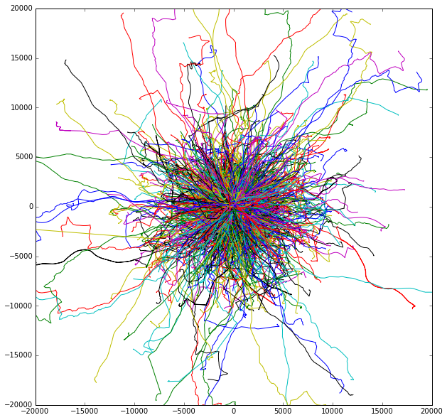
To solve this problem, you first need to come up with signs for machine learning algorithms - something that will distinguish one driver from another. For example, you can take the average speed, average acceleration, etc. For this problem, the selection of descriptive statistics for speed, 1 derivative of speed (acceleration), 2, 3 speeds, and speeds along the main movement — for example, 0, 10, 20 ... 100 percentile for each of the listed distributions, was well suited. Also, the dimensions of the track itself were needed - the maximum and minimum coordinates x, y. This classification problem without a teacher can be reduced to the task of teaching with a teacher by creating a training sample. We will solve the problem individually for each driver: we determine which tracks belong to him and which do not; We know that most of the tracks of his driver belong to him. About the tracks of other drivers, we can confidently say the opposite: they belong to other people. Then mark our own tracks with units (1), and the tracks of other drivers with zeros (0). Thus, we generate a target feature, based on which it is possible to classify tracks as belonging to the driver and not belonging.

Then we will build a random forest model ( RandomForest ) and we will use it as a binary classifier into two classes: 0 and 1. Then, the constructed model is applicable to 200 tracks of the original driver. And the probabilities of the track's belonging to class 1 will be used as an answer. We will repeat this classification for each driver.

Thus, the absence of target features in the set of data analyzed does not mean that we cannot use learning algorithms with a teacher. Depending on the task, we can independently formulate formal criteria for setting the target attribute and create it. This is precisely the analysis of data: in careful and thoughtful work with data and understanding of their nature.

So, the first course is over, the second is in full swing, and we are gaining a third. The start of the third on January 25, 2016 . Recording is open now. Details, as usual, on bigdata.beeline.digital , our official page.