Learn OpenGL. Lesson 6.3 - Image Based Lighting. Diffuse irradiation

Illumination based on the image or IBL ( Image Based Lighting ) - is a category of lighting methods that are not based on analytical light sources (discussed in the previous lesson), but considering the entire environment of the illuminated objects as one continuous source of light. In the general case, the technical basis of such methods lies in processing a cubic map of the environment (prepared in the real world or created on the basis of a three-dimensional scene) so that the data stored in the map can be directly used in lighting calculations: in fact, every texel of the cubic map is considered as a light source . In general, this allows you to capture the effect of global lighting in the scene, which is an important component that conveys the overall “tone” of the current scene and helps the illuminated objects to be better “embedded” in it.

Since IBL algorithms take into account lighting from a certain “global” environment, their result is considered a more accurate simulation of background lighting or even a very rough approximation of global lighting. This aspect makes IBL methods interesting in terms of incorporating the PBR into the model, since using ambient light in the lighting model allows objects to look much more physically correct.


To incorporate the influence of IBL into the already described PBR system, we return to the familiar reflectance equation:

$$

As described earlier, the main goal is to calculate the integral for all incoming radiation directions $$ hemisphere $$. In the last lesson, the calculation of the integral was not burdensome, since we knew in advance the number of light sources, and, therefore, all those several directions of light incidence that correspond to them. At the same time, the integral cannot be solved with a snap: any falling vector$$from the environment can carry non-zero energy brightness. As a result, for the practical applicability of the method it is required to satisfy the following requirements:

• You need to come up with a way to get the energy brightness of the scene for an arbitrary direction vector $$;
• It is necessary that the solution of the integral can occur in real time.

Well, the first point is resolved by itself. A hint of a solution has already slipped here: one of the methods for representing the irradiation of a scene or environment is a cubic map that has undergone special processing. Each texel in such a map can be considered as a separate emitting source. By sampling from such a map according to an arbitrary vector$$we easily get the energy brightness of the scene in this direction.

So, we get the energy brightness of the scene for an arbitrary vector$$:

vec3 radiance = texture(_cubemapEnvironment, w_i).rgb; 

Remarkably, however, solving the integral requires us to make samples from the environment map not from one direction, but from all possible in the hemisphere. And so - for each shaded fragment. Obviously, for real-time tasks this is practically impracticable. A more effective method would be to calculate part of the integrand operations in advance, even outside our application. But for this you will have to roll up your sleeves and dive deeper into the essence of the expression of reflectivity:

$$

It can be seen that the parts of the expression related to the diffuse $$ and mirror $$BRDF components are independent. You can divide the integral into two parts:

$$

Such a division into parts will allow us to deal with each of them individually, and in this lesson we will deal with the part responsible for diffuse lighting.

Having analyzed the form of the integral over the diffuse component, we can conclude that the Lambert diffuse component is essentially constant (color$$refractive index $$ and $$are constant under the conditions of integrand) and does not depend on other variables. Given this fact, we can put the constants beyond the sign of the integral:

$$

So we get an integral depending only on $$ (it is assumed that $$corresponds to the center of the cubic map of the environment). Based on this formula, you can calculate or, even better, pre-calculate a new cubic map that stores the result of calculating the integral of the diffuse component for each direction of the sample (or texel map)$$using the convolution operation.

Convolution is the operation of applying some calculation to each element in a data set, taking into account the data of all other elements in the set. In this case, such data is the energy brightness of the scene or environment map. Thus, to calculate one value in each direction of the sample in the cubic map, we will have to take into account the values ​​taken from all other possible directions of the sample in the hemisphere lying around the sample point.

To convolve the environment map, you need to solve the integral for each resulting direction of the sample$$ by performing multiple discrete samples along directions $$belonging to the hemisphere $$, and averaging the total energy brightness. The hemisphere, on the basis of which the sampling directions are taken$$ oriented along the vector $$representing the destination direction for which the current convolution is being calculated. Look at the picture for a better understanding:



Such a pre-calculated cubic map that stores the integration result for each direction of the sample $$can also be considered as storing the result of summing up all the indirect diffuse illumination in the scene, incident on a certain surface oriented along the direction $$. In other words, such cubic maps are called irradiance maps, because the pre-convolutional cubic environment map allows you to directly sample the amount of irradiation of the scene, coming from an arbitrary direction$$, without additional calculations.

The expression determining the energy brightness also depends on the position of the sampling point $$which we took lying right in the center of the irradiation map. This assumption imposes a limitation in the sense that the source of all indirect diffuse illumination will also be a single environmental map. In scenes that are heterogeneous in lighting, this can destroy the illusion of reality (especially in indoor scenes). Modern rendering engines solve this problem by placing a special helper objects in the scene - the reflection of the sample ( reflection probes ). Each such object is engaged in one task: it forms its own irradiation map for its immediate environment. With this technique, the irradiation (and energy brightness) at an arbitrary point$$will be determined by simple interpolation between the nearest reflection samples. But for current tasks, we agree that the environment map is sampled from its very center, and we will analyze reflection samples in further lessons.

Below is an example of a cubic map of the environment and an irradiation map (based on the wave engine ) derived from it , which averages the energy brightness of the environment for each output direction$$.

So, this card stores the convolution result in each texel (corresponding to the direction $$), and outwardly such a map looks like storing the average color of the environment map. A sample in any direction from such a map will return the value of the irradiation emanating from this direction.

PBR and HDR

In the previous lesson , it was already briefly noted that for the correct operation of the PBR lighting model it is extremely important to take into account the HDR brightness range of the light sources present. Since the PBR model at the input accepts parameters one way or another based on very specific physical quantities and characteristics, it is logical to require that the energy brightness of the light sources matches their real prototypes. It doesn’t matter how we justify the specific value of the radiation flux for each source: make a rough engineering estimate or turn to physical quantities - the difference in characteristics between a room lamp and the sun will be enormous in any case. Without using HDRrange it will be impossible to accurately determine the relative brightness of various light sources.

So, PBR and HDR are friends forever, this is understandable, but how does this fact relate to image-based lighting methods? In the last lesson, it was shown that converting PBR to the HDR rendering range is easy. There remains one “but”: since the indirect illumination from the environment is based on a cubic map of the environment, a way is needed to preserve the HDR characteristics of this background lighting in the environment map.

Until now, we used environment maps created in the LDR format (such as skyboxes , for example) We used the color sample from them in rendering as is and this is quite acceptable for direct shading of objects. And it is completely unsuitable when using environment maps as sources of physically reliable measurements.

RGBE - HDR image format

Get familiar with the RGBE image file format. Files with the extension " .hdr " are used to store images with a wide dynamic range, allocating one byte for each element of the color triad and one more byte for the common exponent. The format also allows you to store cubic environment maps with a color intensity range beyond the LDR range [0., 1.]. This means that light sources can maintain their real intensity, being represented by such an environment map.

The network has quite a lot of free environment maps in RGBE format, shot in various real conditions. Here is an example from the sIBL archive site :


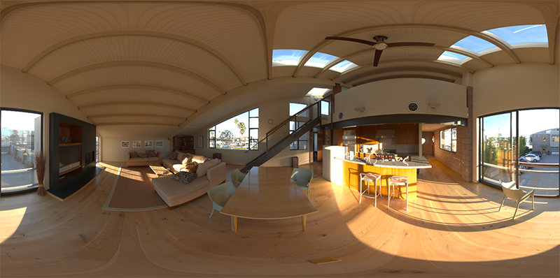
You may be surprised at what you saw: after all, this distorted image does not at all look like a regular cubic map with its pronounced breakdown into 6 faces. The explanation is simple: this map of the environment was projected from a sphere onto a plane - an equal-rectangular scan was applied . This is done to be able to store in a format that does not support the storage mode of cubic cards as is. Of course, this method of projection has its drawbacks: the horizontal resolution is much higher than the vertical. In most cases of application in rendering, this is an acceptable ratio, since usually interesting details of the environment and lighting are located exactly in the horizontal plane, and not in the vertical one. Well, plus to everything, we need the conversion code back to the cubic map.

Support for RGBE format in stb_image.h

Downloading this image format on your own requires knowledge of the format specification , which is not difficult, but still laborious. Fortunately for us , the stb_image.h image loading library , implemented in a single header file, supports loading RGBE files, returning an array of floating-point numbers - what we need for our purposes! Adding a library to your project, loading image data is extremely simple:

#include "stb_image.h"
[...]
stbi_set_flip_vertically_on_load(true);
int width, height, nrComponents;
float *data = stbi_loadf("newport_loft.hdr", &width, &height, &nrComponents, 0);
unsigned int hdrTexture;
if (data)
{
    glGenTextures(1, &hdrTexture);
    glBindTexture(GL_TEXTURE_2D, hdrTexture);
    glTexImage2D(GL_TEXTURE_2D, 0, GL_RGB16F, width, height, 0, GL_RGB, GL_FLOAT, data); 
    glTexParameteri(GL_TEXTURE_2D, GL_TEXTURE_WRAP_S, GL_CLAMP_TO_EDGE);
    glTexParameteri(GL_TEXTURE_2D, GL_TEXTURE_WRAP_T, GL_CLAMP_TO_EDGE);
    glTexParameteri(GL_TEXTURE_2D, GL_TEXTURE_MIN_FILTER, GL_LINEAR);
    glTexParameteri(GL_TEXTURE_2D, GL_TEXTURE_MAG_FILTER, GL_LINEAR);
    stbi_image_free(data);
}
else
{
    std::cout << "Failed to load HDR image." << std::endl;
}  

The library automatically converts values ​​from the internal HDR format to regular real 32-bit numbers, with three color channels by default. It is enough to save the data of the original HDR image in a normal 2D floating-point texture.

Convert an equal-angle scan into a cubic map

An equally rectangular scan can be used to directly select samples from the environment map, however, this would require expensive mathematical operations, while fetching from a normal cubic map would be practically free in performance. It is precisely from these considerations that in this lesson we will deal with the conversion of an equally rectangular image into a cubic map, which will be used later. However, the direct sampling method from an equally rectangular map using a three-dimensional vector will also be shown here, so that you can choose the method of work that suits you.

To convert, you need to draw a unit-sized cube, observing it from the inside, project an equal-rectangular map on its faces, and then extract six images from the faces as the faces of the cubic map. The vertex shader of this stage is quite simple: it simply processes the vertices of the cube as is, and also passes their unreformed positions to the fragment shader for use as a three-dimensional sample vector:

#version 330 core
layout (location = 0) in vec3 aPos;
out vec3 localPos;
uniform mat4 projection;
uniform mat4 view;
void main()
{
    localPos = aPos;  
    gl_Position =  projection * view * vec4(localPos, 1.0);
}

In the fragment shader, we shade each face of the cube as if we were trying to gently wrap the cube with a sheet with an equally rectangular map. To do this, the sample direction transferred to the fragment shader is taken, processed by special trigonometric magic, and, ultimately, the selection is made from an equal-rectangular map as if it were actually a cubic map. The selection result is directly saved as the color of the fragment of the cube face:

#version 330 core
out vec4 FragColor;
in vec3 localPos;
uniform sampler2D equirectangularMap;
const vec2 invAtan = vec2(0.1591, 0.3183);
vec2 SampleSphericalMap(vec3 v)
{
    vec2 uv = vec2(atan(v.z, v.x), asin(v.y));
    uv *= invAtan;
    uv += 0.5;
    return uv;
}
void main()
{		
    // localPos требует нормализации
    vec2 uv = SampleSphericalMap(normalize(localPos)); 
    vec3 color = texture(equirectangularMap, uv).rgb;
    FragColor = vec4(color, 1.0);
}

If you actually draw a cube with this shader and an associated HDR environment map, you get something like this:


Those. it can be seen that in fact we projected a rectangular texture onto a cube. Great, but how will this help us in creating a real cubic map? To end this task, it is necessary to render the same cube 6 times with a camera looking at each of the faces, while writing the output to a separate frame buffer object :

unsigned int captureFBO, captureRBO;
glGenFramebuffers(1, &captureFBO);
glGenRenderbuffers(1, &captureRBO);
glBindFramebuffer(GL_FRAMEBUFFER, captureFBO);
glBindRenderbuffer(GL_RENDERBUFFER, captureRBO);
glRenderbufferStorage(GL_RENDERBUFFER, GL_DEPTH_COMPONENT24, 512, 512);
glFramebufferRenderbuffer(GL_FRAMEBUFFER, GL_DEPTH_ATTACHMENT, GL_RENDERBUFFER, captureRBO); 

Of course, we will not forget to organize the memory for storing each of the six faces of the future cubic map:

unsigned int envCubemap;
glGenTextures(1, &envCubemap);
glBindTexture(GL_TEXTURE_CUBE_MAP, envCubemap);
for (unsigned int i = 0; i < 6; ++i)
{
    // обратите внимание, что каждая грань использует 
    // 16битный формат с плавающей точкой
    glTexImage2D(GL_TEXTURE_CUBE_MAP_POSITIVE_X + i, 0, GL_RGB16F, 
                 512, 512, 0, GL_RGB, GL_FLOAT, nullptr);
}
glTexParameteri(GL_TEXTURE_CUBE_MAP, GL_TEXTURE_WRAP_S, GL_CLAMP_TO_EDGE);
glTexParameteri(GL_TEXTURE_CUBE_MAP, GL_TEXTURE_WRAP_T, GL_CLAMP_TO_EDGE);
glTexParameteri(GL_TEXTURE_CUBE_MAP, GL_TEXTURE_WRAP_R, GL_CLAMP_TO_EDGE);
glTexParameteri(GL_TEXTURE_CUBE_MAP, GL_TEXTURE_MIN_FILTER, GL_LINEAR);
glTexParameteri(GL_TEXTURE_CUBE_MAP, GL_TEXTURE_MAG_FILTER, GL_LINEAR);

After this preparation, it remains only to directly carry out the transfer of parts of an equal-rectangular map on the verge of a cubic map.

We will not go into too much detail, especially since the code repeats much seen in the lessons on the frame buffer and omnidirectional shadows . In principle, it all comes down to preparing six separate view matrices orienting the camera strictly to each of the faces of the cube, as well as a special projection matrix with an angle of view of 90 ° to capture the entire face of the cube. Then, just six times, rendering is performed, and the result is saved in a floating-point framebuffer:

glm::mat4 captureProjection = glm::perspective(glm::radians(90.0f), 1.0f, 0.1f, 10.0f);
glm::mat4 captureViews[] = 
{
   glm::lookAt(glm::vec3(0.0f, 0.0f, 0.0f), glm::vec3( 1.0f,  0.0f,  0.0f), glm::vec3(0.0f, -1.0f,  0.0f)),
   glm::lookAt(glm::vec3(0.0f, 0.0f, 0.0f), glm::vec3(-1.0f,  0.0f,  0.0f), glm::vec3(0.0f, -1.0f,  0.0f)),
   glm::lookAt(glm::vec3(0.0f, 0.0f, 0.0f), glm::vec3( 0.0f,  1.0f,  0.0f), glm::vec3(0.0f,  0.0f,  1.0f)),
   glm::lookAt(glm::vec3(0.0f, 0.0f, 0.0f), glm::vec3( 0.0f, -1.0f,  0.0f), glm::vec3(0.0f,  0.0f, -1.0f)),
   glm::lookAt(glm::vec3(0.0f, 0.0f, 0.0f), glm::vec3( 0.0f,  0.0f,  1.0f), glm::vec3(0.0f, -1.0f,  0.0f)),
   glm::lookAt(glm::vec3(0.0f, 0.0f, 0.0f), glm::vec3( 0.0f,  0.0f, -1.0f), glm::vec3(0.0f, -1.0f,  0.0f))
};
// перевод HDR равнопрямоугольной карты окружения в эквивалентную кубическую карту
equirectangularToCubemapShader.use();
equirectangularToCubemapShader.setInt("equirectangularMap", 0);
equirectangularToCubemapShader.setMat4("projection", captureProjection);
glActiveTexture(GL_TEXTURE0);
glBindTexture(GL_TEXTURE_2D, hdrTexture);
// не забудьте настроить параметры вьюпорта для корректного захвата
glViewport(0, 0, 512, 512);
glBindFramebuffer(GL_FRAMEBUFFER, captureFBO);
for (unsigned int i = 0; i < 6; ++i)
{
    equirectangularToCubemapShader.setMat4("view", captureViews[i]);
    glFramebufferTexture2D(GL_FRAMEBUFFER, GL_COLOR_ATTACHMENT0, 
                           GL_TEXTURE_CUBE_MAP_POSITIVE_X + i, envCubemap, 0);
    glClear(GL_COLOR_BUFFER_BIT | GL_DEPTH_BUFFER_BIT);
    renderCube(); // вывод единичного куба
}
glBindFramebuffer(GL_FRAMEBUFFER, 0);  

Here, the color of the frame buffer is attached, and alternately changing the connected face of the cubic map, which leads to the direct output of the render to one of the faces of the environment map. This code needs to be executed only once, after which we will still have a full-fledged envCubemap environment map containing the result of converting the original equal-rectangular version of the HDR environment map.

We will test the resulting cubic map by sketching the simplest skybox shader:

#version 330 core
layout (location = 0) in vec3 aPos;
uniform mat4 projection;
uniform mat4 view;
out vec3 localPos;
void main()
{
    localPos = aPos;
    // здесь отбрасываем данные о переносе из видовой матрицы
    mat4 rotView = mat4(mat3(view));
    vec4 clipPos = projection * rotView * vec4(localPos, 1.0);
    gl_Position = clipPos.xyww;
}

Pay attention to the trick with the components of the clipPos vector : we use the xyww tetrad when recording the transformed coordinate of the vertex to ensure that all fragments of the skybox have a maximum depth of 1.0 (the approach was already used in the corresponding lesson ). Do not forget to change the comparison function to GL_LEQUAL :

glDepthFunc(GL_LEQUAL); 

The fragment shader simply selects from a cubic map:

#version 330 core
out vec4 FragColor;
in vec3 localPos;
uniform samplerCube environmentMap;
void main()
{
    vec3 envColor = texture(environmentMap, localPos).rgb;
    envColor = envColor / (envColor + vec3(1.0));
    envColor = pow(envColor, vec3(1.0/2.2)); 
    FragColor = vec4(envColor, 1.0);
}

The selection from the map is based on the interpolated local coordinates of the vertices of the cube, which is the correct direction of the selection in this case (again, discussed in the lesson on skyboxes, approx. Per. ). Since the transport components in the view matrix were ignored, the render of the skybox will not depend on the position of the observer, creating the illusion of an infinitely distant background. Since here we directly output data from the HDR card to the default framebuffer, which is the LDR receiver, it is necessary to recall the tonal compression. And finally, almost all HDR cards are stored in linear space, which means that gamma correction must be applied as the final processing chord.

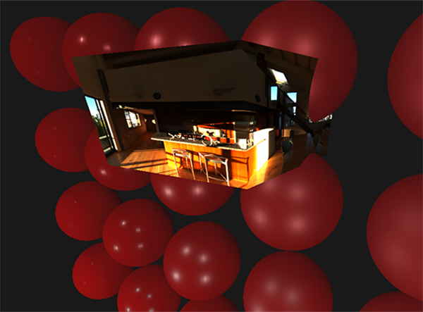
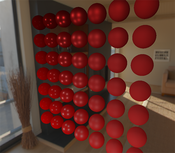
So, when outputting the obtained skybox, along with the already familiar array of spheres, something similar is obtained:


Well, a lot of effort was spent, but in the end we successfully got used to reading the HDR environment map, converting it from an equilateral to a cubic map, and outputting the HDR cubic map as a skybox in the scene. Moreover, the code for converting to a cubic map by rendering to six faces of a cubic map is useful to us further on in the task of convolution of an environment map . The code for the entire conversion process is here .

Convolution of a cubic card

As was said at the beginning of the lesson, our main goal is to solve the integral for all possible directions of indirect diffuse lighting, taking into account the given irradiation of the scene in the form of a cubic map of the environment. It is known that we can get the value of the energy brightness of the scene$$ for arbitrary direction $$by sampling from the HDR a cubic map of the environment in that direction. To solve the integral, it will be necessary to sample the energy brightness of the scene from all possible directions in the hemisphere$$each reviewed fragment.
Obviously, the task of sampling lighting from the environment from all possible directions in the hemisphere$$is computationally impracticable - there are an infinite number of such directions. However, it is possible to apply the approximation by taking a finite number of directions chosen randomly or located uniformly inside the hemisphere. This will allow us to obtain a fairly good approximation to true irradiation, essentially solving the integral of interest to us in the form of a finite sum.

But for real-time tasks, even such an approach is still incredibly imposed, because the samples are taken for each fragment, and the number of samples must be high enough for an acceptable result. So it would be nice to prepare in advanceThe data for this step is outside the rendering process. Since the orientation of the hemisphere determines from which region of space we capture the irradiation, we can pre-calculate the irradiation for each possible orientation of the hemisphere based on all possible outgoing directions$$:

$$

As a result, for a given arbitrary vector $$, we can sample from the calculated irradiance map in order to obtain the diffuse irradiance in this direction. To determine the magnitude of indirect diffuse radiation at the point of the current fragment, we take the total irradiation from a hemisphere oriented along the normal to the fragment surface. In other words, obtaining the irradiation of a scene comes down to a simple selection:

 vec3 irradiance = texture(irradianceMap, N);

Further, to create an irradiation map, it is necessary to convolve the environment map, converted to a cubic map. We know that for each fragment its hemisphere is considered oriented along the normal to the surface$$. In this case, the convolution of the cubic map is reduced to calculating the average amount of energy brightness from all directions$$ inside the hemisphere $$oriented along the normal $$:


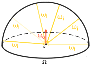
Fortunately, the time-consuming preliminary work that we did at the beginning of the lesson will now make it quite easy to convert the environment map into a cubic map in a special fragment shader, the output of which will be used to form a new cubic map. For this, the very piece of code that was used to translate an equal-rectangular environment map into a cubic map is useful.

It remains only to take another processing shader:

#version 330 core
out vec4 FragColor;
in vec3 localPos;
uniform samplerCube environmentMap;
const float PI = 3.14159265359;
void main()
{		
    // направление выборки идентично направлению ориентации полусферы
    vec3 normal = normalize(localPos);
    vec3 irradiance = vec3(0.0);
    [...] // код свертки
    FragColor = vec4(irradiance, 1.0);
}

Here, the environmentMap sampler is an HDR cubic map of the environment previously derived from an equilateral.

There are many ways to convolve the environment map. In this case, for each texel of the cubic map, we will generate several hemisphere sample vectors$$oriented along the direction of the sample, and average the results. The number of sample vectors will be fixed, and the vectors themselves will be evenly distributed within the hemisphere. I note that the integrand is a continuous function, and a discrete estimate of this function will be only an approximation. And the more sampling vectors we take, the closer to the analytical solution of the integral we will be.

The integrand of the expression for reflectivity depends on the solid angle$$- values ​​with which it is not very convenient to work. Instead of integrating over a solid angle$$ we will change the expression, leading to integration over spherical coordinates $$ and $$:


The angle Phi will represent the azimuth in the plane of the base of the hemisphere, varying from 0 to $$. Angle$$ will represent the elevation angle, varying from 0 to $$. The modified expression for reflectivity in such terms is as follows:

$$

The solution of such an integral will require taking a finite number of samples in the hemisphere $$and averaging the results. Knowing the number of samples$$ and $$over each of the spherical coordinates, we can translate the integral to the Riemannian sum :

$$

Since both spherical coordinates vary discretely, at each moment, sampling is performed with a certain averaged area in the hemisphere, as can be seen in the figure above. Due to the nature of the spherical surface, the size of the discrete sampling area inevitably decreases with increasing elevation angle$$and approaching the zenith. To compensate for this effect of reducing the area, we added a weight coefficient to the expression$$.

As a result, the implementation of discrete sampling in the hemisphere based on spherical coordinates for each fragment in the form of code is as follows:

vec3 irradiance = vec3(0.0);  
vec3 up    = vec3(0.0, 1.0, 0.0);
vec3 right = cross(up, normal);
up         = cross(normal, right);
float sampleDelta = 0.025;
float nrSamples = 0.0; 
for(float phi = 0.0; phi < 2.0 * PI; phi += sampleDelta)
{
    for(float theta = 0.0; theta < 0.5 * PI; theta += sampleDelta)
    {
        // перевод сферических коорд. в декартовы (в касательном пр-ве)
        vec3 tangentSample = vec3(sin(theta) * cos(phi),  sin(theta) * sin(phi), cos(theta));
        // из касательного в мировое пространство
        vec3 sampleVec = tangentSample.x * right + tangentSample.y * up + tangentSample.z * N; 
        irradiance += texture(environmentMap, sampleVec).rgb * cos(theta) * sin(theta);
        nrSamples++;
    }
}
irradiance = PI * irradiance * (1.0 / float(nrSamples));

The variable sampleDelta determines the size of the discrete step along the surface of the hemisphere. By changing this value, you can increase or decrease the accuracy of the result.

Inside both cycles, a regular 3-dimensional sample vector is formed from spherical coordinates, transferred from tangent to world space, and then used to sample a cubic environment map from the HDR. The result of the samples is accumulated in the irradiance variable , which at the end of the processing will be divided by the number of samples made in order to obtain an average value of irradiation. Note that the result of sampling from the texture is modulated by two quantities: cos (theta) - to take into account the attenuation of light at large angles, and sin (theta)- to compensate for the reduction in sample area when approaching the zenith.

It remains only to deal with the code that renders and captures the results of the convolution of the envCubemap environment map . First, create a cubic map to store the irradiation (you will need to do it once, before entering the main render cycle):

unsigned int irradianceMap;
glGenTextures(1, &irradianceMap);
glBindTexture(GL_TEXTURE_CUBE_MAP, irradianceMap);
for (unsigned int i = 0; i < 6; ++i)
{
    glTexImage2D(GL_TEXTURE_CUBE_MAP_POSITIVE_X + i, 0, GL_RGB16F, 32, 32, 0, 
                 GL_RGB, GL_FLOAT, nullptr);
}
glTexParameteri(GL_TEXTURE_CUBE_MAP, GL_TEXTURE_WRAP_S, GL_CLAMP_TO_EDGE);
glTexParameteri(GL_TEXTURE_CUBE_MAP, GL_TEXTURE_WRAP_T, GL_CLAMP_TO_EDGE);
glTexParameteri(GL_TEXTURE_CUBE_MAP, GL_TEXTURE_WRAP_R, GL_CLAMP_TO_EDGE);
glTexParameteri(GL_TEXTURE_CUBE_MAP, GL_TEXTURE_MIN_FILTER, GL_LINEAR);
glTexParameteri(GL_TEXTURE_CUBE_MAP, GL_TEXTURE_MAG_FILTER, GL_LINEAR);

Since the irradiation map is obtained by averaging uniformly distributed samples of the energy brightness of the environment map, it practically does not contain high-frequency parts and elements - a fairly small resolution texture (32x32 here) and enabled linear filtering will be enough to store it.

Next, set the capture framebuffer to this resolution:

glBindFramebuffer(GL_FRAMEBUFFER, captureFBO);
glBindRenderbuffer(GL_RENDERBUFFER, captureRBO);
glRenderbufferStorage(GL_RENDERBUFFER, GL_DEPTH_COMPONENT24, 32, 32);  

The code for capturing the convolution results is similar to the code for transferring an environment map from an equilateral to a cubic one, only a convolution shader is used:

irradianceShader.use();
irradianceShader.setInt("environmentMap", 0);
irradianceShader.setMat4("projection", captureProjection);
glActiveTexture(GL_TEXTURE0);
glBindTexture(GL_TEXTURE_CUBE_MAP, envCubemap);
// не забудьте настроить вьюпорт под захватываемый размер
glViewport(0, 0, 32, 32);
glBindFramebuffer(GL_FRAMEBUFFER, captureFBO);
for (unsigned int i = 0; i < 6; ++i)
{
    irradianceShader.setMat4("view", captureViews[i]);
    glFramebufferTexture2D(GL_FRAMEBUFFER, GL_COLOR_ATTACHMENT0, 
                           GL_TEXTURE_CUBE_MAP_POSITIVE_X + i, irradianceMap, 0);
    glClear(GL_COLOR_BUFFER_BIT | GL_DEPTH_BUFFER_BIT);
    renderCube();
}
glBindFramebuffer(GL_FRAMEBUFFER, 0);  

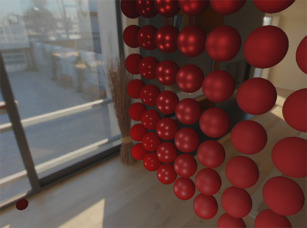
After completing this stage, we will have a pre-calculated irradiation map on our hands that can be directly used to calculate indirect diffuse illumination. To check how the convolution went, we’ll try to replace the skybox texture from the environment map with the irradiation map:


If, as a result, you saw something that looked like a very blurry map of the environment, then, most likely, the convolution was successful.

PBR and indirect illumination

The resulting irradiation map is used in the diffuse part of the divided expression of reflectivity and represents the accumulated contribution from all possible directions of indirect illumination. Since in this case the light does not come from specific sources, but from the environment as a whole, we consider diffuse and mirror indirect lighting as background ( ambient ), replacing the previously used constant value.

To begin with, do not forget to add a new sampler with an irradiation map:

uniform samplerCube irradianceMap;

Having an irradiation map that stores all the information about indirect diffuse radiation from the scene and normal to the surface, obtaining data on the irradiation of a particular fragment is as simple as making one sample from the texture:

// vec3 ambient = vec3(0.03);
vec3 ambient = texture(irradianceMap, N).rgb;

However, since indirect radiation contains data for both the diffuse and mirror components (as we saw in the component version of the expression of reflectivity), we need to modulate the diffuse component in a special way. As in the previous lesson, we use the Fresnel expression to determine the degree of reflection of light for a given surface, whence we obtain the degree of refraction of light or the diffuse coefficient:

vec3 kS = fresnelSchlick(max(dot(N, V), 0.0), F0);
vec3 kD = 1.0 - kS;
vec3 irradiance = texture(irradianceMap, N).rgb;
vec3 diffuse    = irradiance * albedo;
vec3 ambient    = (kD * diffuse) * ao; 

As background lighting falls from all directions in the hemisphere based on the normal to the surface $$, it is impossible to determine a single median ( halfway) vector for calculating the Fresnel coefficient. In order to simulate the Fresnel effect under such conditions, it is necessary to calculate the coefficient based on the angle between the normal and the observation vector. However, earlier, as a parameter for calculating the Fresnel coefficient, we used the median vector obtained on the basis of the model of microsurfaces and depending on the surface roughness. Since in this case, the roughness is not included in the calculation parameters, the degree of reflection of light by the surface will always be overestimated. Indirect lighting as a whole should behave the same as direct lighting, i.e. from rough surfaces we expect a lower degree of reflection at the edges. But since the roughness is not taken into account,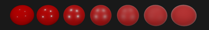


You can get around this nuisance by introducing roughness into the Fremlin-Schlick expression, a process described by Sébastien Lagarde :

vec3 fresnelSchlickRoughness(float cosTheta, vec3 F0, float roughness)
{
    return F0 + (max(vec3(1.0 - roughness), F0) - F0) * pow(1.0 - cosTheta, 5.0);
}

Given the surface roughness when calculating the Fresnel set, the code for calculating the background component takes the following form:

vec3 kS = fresnelSchlickRoughness(max(dot(N, V), 0.0), F0, roughness); 
vec3 kD = 1.0 - kS;
vec3 irradiance = texture(irradianceMap, N).rgb;
vec3 diffuse    = irradiance * albedo;
vec3 ambient    = (kD * diffuse) * ao; 

As it turned out, the use of image-based lighting inherently boils down to one sample from a cubic map. All difficulties are mainly associated with the preliminary preparation and transfer of the environment map to the irradiation map.

Taking a familiar scene from a lesson on analytical light sources containing an array of spheres with varying metallicity and roughness, and adding diffuse background lighting from the environment, you get something like this:


It still looks strange, since materials with a high degree of metallicity still require reflection in order to really look, hmm, metal (metals do not reflect diffuse lighting, after all). And in this case, the only reflections obtained from point analytical light sources. And yet, we can already say that the spheres look more immersed in the environment (especially noticeable when switching environment maps), since the surfaces now correctly respond to background lighting from the scene environment.

The full source code for the lesson is here.. In the next lesson, we will finally deal with the second half of the expression of reflectivity, which is responsible for indirect specular lighting. After this step, you will truly feel the power of the PBR approach in lighting.

Additional materials

• Coding Labs: Physically based rendering : an introduction to the PBR model along with an explanation of how the irradiance map is constructed and why.
• The Mathematics of Shading : A brief overview from ScratchAPixel on some of the mathematical techniques used in this lesson, in particular about polar coordinates and integrals.

PS : We have a telegram conf for coordination of transfers. If you have a serious desire to help with the translation, then you are welcome!