OpenEMS modeling basics
In the last part, it was described how to install and configure the open-source electromagnetic simulator openEMS . Now you can move on to modeling. How to make EMF simulations using openEMS and Octave will be described in this article.
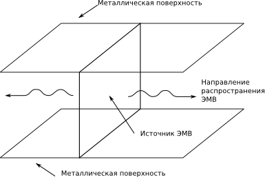
We will simulate the process of propagation of an electromagnetic wave (EMW) between two parallel metal plates.
The configuration of the object is shown in the figure. A rectangular source of EMW is assumed, from which EMW propagates in both directions.
Below the cat is a line-by-line parsing of a script for modeling such an object.
As mentioned in the previous part, all simulations in openEMS are Octave / Matlab scripts. Run Octave / Matlab and enter the following commands. Initialize the space first. We create a special FDTD object that describes the space of finite difference in the time domain:
Function parameters are 100 points of calculation in time from zero. The time step is automatically selected based on the Nyquist frequency and the frequency of the EMW source. Try to set a different number of points, for example 1000.
Now we set the source of electromagnetic waves with a frequency of 10 MHz. Here the function parameters are clear from the name.
For any simulation of electromagnetic waves, boundary conditions are needed. The boundary conditions describe the properties of the material, which is limited to the spaces in the direction of each of the three coordinate axes X, Y, Z. The order of the boundary conditions in the parameters of the function is as follows X +, X-, Y +, Y-, Z +, Z-. Our space along the Y axis in the positive direction is limited by a perfectly conducting surface (PEC - Perfect Electric Conductor), in the negative direction along Y - also conductive surface. PMC is an ideal
magnetic conductor. MUR is an absolutely absorbing dielectric. It approximately corresponds to the material of the walls of the anechoic chamber.
A special multilayer material (PML_x) is also available for boundary conditions. It can have from 6 to 20 layers (for example PML_8, PML_10). This material also acts as an absorbing dielectric.
After the boundary conditions are set, we initialize the CSX space in which the geometry of our system will be set.
Now you need to create a grid. The calculation of the propagation of electromagnetic waves will be performed inside the space limited by the grid. First, set the grid dimension by coordinates (X * Y * Z = 20x20 * 40 meters).
Now we create the grid itself in rectangular coordinates using the
DefineRectGrid () function and apply it to the geometry (the grid step is 1 meter):
Next, we create a source of EMW. We set the amplitude of the electromagnetic wave and the direction of the vector of electromagnetic wave. To do this, use the AddExcitation function.
The first and second parameters of the function are the name of the CSX space and the name of the source of the electromagnetic wave, respectively. The third parameter of the function is the type of field. The following types are available:
The difference between hard and soft excitation is that with hard excitation, the EMW amplitude at a given point in space is set to a forced value, and with soft excitation, the superposition of the fields is calculated, that is, EMW is superimposed on the fields available at this point in space.
The fourth parameter is a vector whose components specify the amplitude of the EMW in three directions X, Y, Z.
Thus, we set the excitation by an electric field with an amplitude of 1 V / m in the direction of the Y axis.
Now we create a platform (AddBox) from which EMW will propagate. This site is actually the source of EMW.
This completes the description of the geometry. After we have described the geometry, we need to create a section in which we will observe the propagation of electromagnetic waves. This is done using the AddDump () and AddBox () functions.
Now we are preparing a temporary directory for storing calculation results and viewing the geometry using CSXCAD.
Everything, the model of our structure is ready. You can run the simulator. If everything is fine, then we will see the following report:
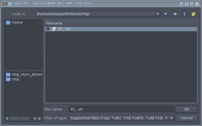
The simulation is complete and you can view the result. Launch Paraview. Then select File-> Open and go to the temporary directory where the simulation results are stored. There we open the file Et_.vtr. This file contains information about the result of calculating the process of EMW propagation in time. Here's what you need to open, the path to the file you will have is different:
Now we see in the Paraview window a plane, which is the section in which we look at the amplitude of the EMW.

To visualize the amplitude of electromagnetic waves, you need to select E-field in the Coloring drop-down list (SolidColor is there by default) and then display the color legend (click Show). Now we see the amplitude of the EMW at time t = 0. At the initial moment of time, the amplitude of the EMW is also equal to zero in all space, so the entire plane will be painted over in one color. To see the EMV distribution, you need to set a time other than zero and press the Rescale button. Now on the plane the EMF amplitude distribution will be displayed.
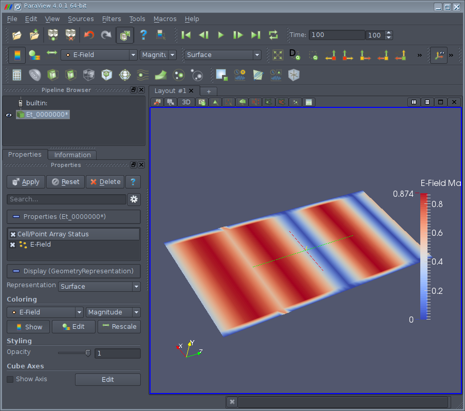
You can also start the animation and view the process of EMW propagation in time. As expected, EMW propagates in both directions from the source plane.
As a result, we simulated in the time domain the process of EMW propagation in a certain region of space. In conclusion, the entire Octave / Matlab script:
Link to previous openEMS article: habrahabr.ru/post/255317
openEMS project website: openems.de
We will simulate the process of propagation of an electromagnetic wave (EMW) between two parallel metal plates.
The configuration of the object is shown in the figure. A rectangular source of EMW is assumed, from which EMW propagates in both directions.
Below the cat is a line-by-line parsing of a script for modeling such an object.
As mentioned in the previous part, all simulations in openEMS are Octave / Matlab scripts. Run Octave / Matlab and enter the following commands. Initialize the space first. We create a special FDTD object that describes the space of finite difference in the time domain:
FDTD = InitFDTD('NrTS',100,'EndCriteria',0,'OverSampling',50);
Function parameters are 100 points of calculation in time from zero. The time step is automatically selected based on the Nyquist frequency and the frequency of the EMW source. Try to set a different number of points, for example 1000.
Now we set the source of electromagnetic waves with a frequency of 10 MHz. Here the function parameters are clear from the name.
FDTD = SetSinusExcite(FDTD,10e6);
For any simulation of electromagnetic waves, boundary conditions are needed. The boundary conditions describe the properties of the material, which is limited to the spaces in the direction of each of the three coordinate axes X, Y, Z. The order of the boundary conditions in the parameters of the function is as follows X +, X-, Y +, Y-, Z +, Z-. Our space along the Y axis in the positive direction is limited by a perfectly conducting surface (PEC - Perfect Electric Conductor), in the negative direction along Y - also conductive surface. PMC is an ideal
magnetic conductor. MUR is an absolutely absorbing dielectric. It approximately corresponds to the material of the walls of the anechoic chamber.
FDTD = SetBoundaryCond(FDTD,{'PMC' 'PMC' 'PEC' 'PEC' 'MUR' 'MUR'});
A special multilayer material (PML_x) is also available for boundary conditions. It can have from 6 to 20 layers (for example PML_8, PML_10). This material also acts as an absorbing dielectric.
After the boundary conditions are set, we initialize the CSX space in which the geometry of our system will be set.
CSX = InitCSX();
Now you need to create a grid. The calculation of the propagation of electromagnetic waves will be performed inside the space limited by the grid. First, set the grid dimension by coordinates (X * Y * Z = 20x20 * 40 meters).
mesh.x = -10:10;
mesh.y = -10:10;
mesh.z = -10:30;
Now we create the grid itself in rectangular coordinates using the
DefineRectGrid () function and apply it to the geometry (the grid step is 1 meter):
CSX = DefineRectGrid(CSX,1,mesh);
Next, we create a source of EMW. We set the amplitude of the electromagnetic wave and the direction of the vector of electromagnetic wave. To do this, use the AddExcitation function.
CSX = AddExcitation(CSX,'excitation',0,[0 1 0]);
The first and second parameters of the function are the name of the CSX space and the name of the source of the electromagnetic wave, respectively. The third parameter of the function is the type of field. The following types are available:
- 0 - electric field (E), hard excitation
- 1 - electric field (E), hard excitation
- 2 - magnetic field (N), soft excitation
- 3 - magnetic field (P), hard excitation
- 10 - flat EMV
The difference between hard and soft excitation is that with hard excitation, the EMW amplitude at a given point in space is set to a forced value, and with soft excitation, the superposition of the fields is calculated, that is, EMW is superimposed on the fields available at this point in space.
The fourth parameter is a vector whose components specify the amplitude of the EMW in three directions X, Y, Z.
Thus, we set the excitation by an electric field with an amplitude of 1 V / m in the direction of the Y axis.
Now we create a platform (AddBox) from which EMW will propagate. This site is actually the source of EMW.
CSX = AddBox(CSX,'excitation',0,[-10 -10 0],[10 10 0]);
This completes the description of the geometry. After we have described the geometry, we need to create a section in which we will observe the propagation of electromagnetic waves. This is done using the AddDump () and AddBox () functions.
CSX = AddDump(CSX,'Et');
CSX = AddBox(CSX,'Et',0,[-10 0 -10],[10 0 30]);
Now we are preparing a temporary directory for storing calculation results and viewing the geometry using CSXCAD.
mkdir('tmp');
WriteOpenEMS('/tmp/tmp.xml',FDTD,CSX);
CSXGeomPlot('/tmp/tmp.xml');
invoking AppCSXCAD, exit to continue script...
QCSXCAD - disabling editing
Everything, the model of our structure is ready. You can run the simulator. If everything is fine, then we will see the following report:
RunOpenEMS('tmp','/tmp/tmp.xml','');
 ----------------------------------------------------------------------
 | openEMS 64bit -- version v0.0.32-14-g63adb58
 | (C) 2010-2013 Thorsten Liebig   GPL license
 ----------------------------------------------------------------------
        Used external libraries:
                CSXCAD -- Version: v0.5.2-15-gcb5b3cf
                hdf5   -- Version: 1.8.13
                          compiled against: HDF5 library version: 1.8.13
                tinyxml -- compiled against: 2.6.2
                fparser
                boost  -- compiled against: 1_54
                vtk -- Version: 5.10.1
                       compiled against: 5.10.1
Create FDTD operator (compressed SSE + multi-threading)
FDTD simulation size: 21x21x41 --> 18081 FDTD cells
FDTD timestep is: 1.92583e-09 s; Nyquist rate: 25 timesteps @1.03851e+07 Hz
Excitation signal length is: 100 timesteps (1.92583e-07s)
Max. number of timesteps: 100 ( --> 1 * Excitation signal length)
Create FDTD engine (compressed SSE + multi-threading)
Running FDTD engine... this may take a while... grab a cup of coffee?!?
Time for 100 iterations with 18081 cells : 0.1624 sec
Speed: 11.1336 MCells/s
The simulation is complete and you can view the result. Launch Paraview. Then select File-> Open and go to the temporary directory where the simulation results are stored. There we open the file Et_.vtr. This file contains information about the result of calculating the process of EMW propagation in time. Here's what you need to open, the path to the file you will have is different:
Now we see in the Paraview window a plane, which is the section in which we look at the amplitude of the EMW.
To visualize the amplitude of electromagnetic waves, you need to select E-field in the Coloring drop-down list (SolidColor is there by default) and then display the color legend (click Show). Now we see the amplitude of the EMW at time t = 0. At the initial moment of time, the amplitude of the EMW is also equal to zero in all space, so the entire plane will be painted over in one color. To see the EMV distribution, you need to set a time other than zero and press the Rescale button. Now on the plane the EMF amplitude distribution will be displayed.
You can also start the animation and view the process of EMW propagation in time. As expected, EMW propagates in both directions from the source plane.
As a result, we simulated in the time domain the process of EMW propagation in a certain region of space. In conclusion, the entire Octave / Matlab script:
FDTD = InitFDTD('NrTS',1000,'EndCriteria',0,'OverSampling',1);
FDTD = SetSinusExcite(FDTD,10e6);
FDTD = SetBoundaryCond(FDTD,{'PMC' 'PMC' 'PEC' 'PEC' 'MUR' 'MUR'});
CSX = InitCSX();
mesh.x = -10:10;
mesh.y = -10:10;
mesh.z = -10:30;
CSX = DefineRectGrid(CSX,1,mesh);
CSX = AddExcitation(CSX,'excitation',0,[0 1 0]);
CSX = AddBox(CSX,'excitation',0,[-10 -10 0],[10 10 0]);
CSX = AddDump(CSX,'Et');
CSX = AddBox(CSX,'Et',0,[-10 0 -10],[10 0 30]);
mkdir('tmp');
WriteOpenEMS('/tmp/tmp.xml',FDTD,CSX);
CSXGeomPlot('/tmp/tmp.xml');
RunOpenEMS('tmp','/tmp/tmp.xml','');
Link to previous openEMS article: habrahabr.ru/post/255317
openEMS project website: openems.de