Learn OpenGL. Lesson 6.1. PBR or Physically-correct rendering. Theory

Physically correct rendering

PBR, or physically-correct rendering (physically-based rendering), is a set of visualization techniques based on a theory that agrees fairly well with the real theory of light propagation. Since the goal of PBR is a physically accurate imitation of light, it looks much more realistic than the Phong and Blinna-Phong lighting models we used earlier. It not only looks better, but also gives a good approximation to real physics, which allows us (and, in particular, artists) to create materials based on the physical properties of surfaces, without resorting to cheap tricks to make the lighting look realistic. The main advantage of this approach is that the materials we create will look as intended regardless of the lighting conditions, which is not the case with other non-PBR approaches.

However, PBR is still an approximation of reality (based on the laws of physics), so it is called physical-correct rendering, not physical rendering. In order for a lighting model to be called physically correct, it must meet 3 conditions (don't worry, we'll get to them soon):

• Build on reflective micro-face models
• Obey the law of conservation of energy
• Use the two-beam reflectance function (eng. Bidirectional reflectance distribution function - BRDF)

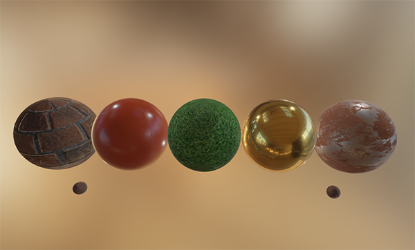
In this series of tutorials, we will focus on the PBR approach, originally developed at Disney and adapted for real-time visualization by Epic Games. Their approach, based on the metal-dielectric working process (the English metallic workflow, did not find a better translation - approx. Ed. ), Is well-documented, widely accepted in many popular engines, and looks amazing. At the end of this section, we get something like this:

Keep in mind that the articles in this section are quite advanced, so it is recommended to have a good understanding of OpenGL and shader lighting. Here are some of the knowledge you will need to study this section: frame buffer , cubic maps , gamma correction , HDR and normal maps . We will also delve a bit into mathematics, but I promise to do everything possible to explain everything as clearly as possible.

Model of reflective micro-facets

All PBR techniques are based on the theory of microfaces. This theory says that each surface with a strong magnification can be represented as a set of microscopic mirrors, called microfaces . Due to the surface roughness of these micro-mirrors can be oriented in different directions:

The more rough the surface, the more chaotically oriented its microgranes. The result of this arrangement of these small mirrors is (in particular when it comes to specular highlights and reflections) that the incident rays of light are scattered in different directions on rough surfaces, which leads to a wider specular reflector. And vice versa: on smooth surfaces, the incident rays are more likely to reflect in one direction, which will give a smaller and sharper flare:

At the microscopic level, there are no absolutely smooth surfaces, but given the fact that the microfaces are rather small and we cannot distinguish between them within our pixel space, we statistically approximate the surface roughness by introducing the roughness coefficient . Using this coefficient, we can calculate the fraction of microfaces oriented in the direction of some vector$$. This vector$$ nothing more than a median vector lying in the middle between the direction of the incident light $$ and the direction of the observer $$. We talked about it earlier, in the lesson on advanced lighting , where we defined it as the ratio of the sum of vectors$$ and $$ to the length of the resulting vector:

$$

The more microfaces are oriented in the direction of the median vector, the sharper and brighter the specular highlight will be. Due to the roughness coefficient, which lies between 0 and 1, we can statistically approximate the orientation of the micro-facets:

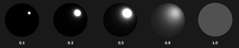
As can be seen, a higher value of the roughness coefficient gives a larger specular highlight stain, compared with a small and sharp spot on smooth surfaces.

Energy saving.

The use of the approximation taking into account the microfaces already carries some form of energy conservation: the energy of the reflected light will never exceed the energy of the incident (if the surface does not glow by itself). Looking at the image above, we see that as the surface roughness increases, the spot of the reflected light increases, but at the same time its brightness decreases. If the intensity of the reflected light were the same for all pixels, regardless of the size of the spot, then rougher surfaces would emit much more energy, which would violate the law of conservation of energy. Therefore, specular reflections are brighter on smooth surfaces and dull on rough ones.

In order for energy to be conserved, we must make a clear separation between the diffuse and specular components. At that moment when the light beam reaches the surface, it is divided into reflected and refracted components. The reflected component is light that is reflected directly, and does not penetrate the surface, we know it as a specular component of light. The refracted component is a light that penetrates into the surface and is absorbed by it — it is known to us as the diffuse component of light.

But there are some nuances associated with the absorption of light - it does not happen instantly as soon as the light touches the surface. From the physics course, we know that light can be described as a beam of photons with energy that moves in a straight line until it loses all energy as a result of a collision with obstacles. Each material consists of microparticles that can interact with a ray of light, as shown in the figure below. These particles absorb some or all of the light energy at each collision, converting it into heat.

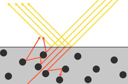
In general, not all of the energy is absorbed, and the light continues to be scattered in (mostly) random directions, where it collides with other particles again until it dries up, or it leaves the surface again. Thus, the surface begins to re-emit light rays, making a contribution in the form of the observed (diffuse) color of the surface. Using PBR, we make a simplified assumption that all the refracted light is absorbed and scattered over a small area of ​​impact, ignoring the effect of scattered light that leaves the surface at a distance from this area. Special shader techniques that take this into account are known as subsurface scattering techniques ., significantly improve the visual quality of materials like leather, marble, wax, but are expensive in terms of performance.

Additional subtleties appear with the refraction and reflection of light on metal surfaces. Metallic surfaces otherwise interact with light than non-metallic (i.e. dielectrics). They obey the same laws of refraction and reflection, with one exception: all the refracted light is absorbed by the surface without scattering, only the specularly reflected light remains; in other words, metal surfaces do not have a diffuse color. Because of this obvious difference between metals and dielectrics, they will be processed differently in the PBR pipeline into which we will delve further along the course of the article.

This difference between reflected and refracted light leads us to another observation regarding the conservation of energy: their values ​​are mutually exclusive. The energy of the reflected light cannot be absorbed by the material. Therefore, the energy absorbed by the surface in the form of refracted light is the remaining energy after taking into account the reflected.
We use this ratio by first calculating the reflected part as a percentage of the energy of the incident rays reflected by the surface, and then the fraction of the refracted light directly from the reflected light, like:

float kS = calculateSpecularComponent(...); // отраженная/зеркальная часть
float kD = 1.0 - kS;                        // преломленная/диффузная часть

In this way we will know the values ​​of both the reflected and refracted parts due to the law of conservation of energy. With this approach, neither the refracted (diffuse) nor the reflected part will exceed 1.0, ensuring that their total energy does not exceed the value of the energy of the incident light, which we could not take into account in previous lessons.

Reflection equation

The above brings us to the so-called rendering equation : a complex equation, invented by very smart guys, and today the best model to simulate lighting. PBR strictly follows a more specific version of this equation, known as the reflection equation . In order to understand PBR well, it is important to first have a thorough understanding of the reflection equation:

$$

At first, it looks frightening, but we will sort it out gradually, piece by piece, and you will see how slowly it will begin to make sense. To understand this equation we will have to delve a little into radiometry. Radiometry- This is the science of measuring electromagnetic radiation (including visible light). There are several radiometric quantities that we can use to measure illumination, but we will only use one relating to the reflection equation, known as Energy Brightness (eng. Radiance) and denoted here by the letter L. HP is used to quantify the magnitude or intensity of light, coming from a certain direction. EH, in turn, is a combination of several physical quantities, and to make it easier for us to imagine it, we will focus on each of them separately.

Radiation flux (English radiant flux)

Radiation flux ($$) is the power of light transmitted energy, measured in watts. The total light energy is made up of a set of terms for different wavelengths, each of which has its own color spectrum. The energy emitted by the light source, in this case, can be represented as a function of all these wavelengths. Wavelengths from 390nm to 700nm make up the visible part of the spectrum, that is, radiation in this range can be perceived by the human eye. In the image below you can see the energy values ​​for the different wavelengths of daylight:

The radiation flux corresponds to the area under the graph of this function from all wavelengths. Directly using the wavelengths of light as input data in computer graphics is impractical, so we resort to a simplified representation of the radiation flux using a triple of colors instead of a function of all wavelengths, known as RGB (or as we usually call it - lighting color). Such a presentation leads to some loss of information, but in general this will have a slight effect on the final picture.

Solid angle (English solid angle)

Solid angle , denoted as$$gives us the size or area of ​​a figure projected onto a single sphere. You can present it as a direction having a volume of:

Imagine that you are in the center of a sphere and look in the direction of a figure. The size of the resulting silhouette will be a solid angle.

Radiation intensity (eng. Radiance intensity)

The radiation force measures the amount of radiation flux per solid angle, or the power of a light source per square of a unit sphere defined by a solid angle. For example, for an omnidirectional light source that radiates equally in all directions, the radiation power means the light energy per specific area (solid angle):

The equation describing the strength of the radiation looks like this:

$$

where I is the radiation flux Φ falling on the solid angle$$

Knowing the radiation flux, the force and the solid angle, we can describe the energy brightness equation that describes the total observed energy in area A, limited by the solid angle O for light by force $$

$$

Energy brightness is the radiometric amount of light in an area that depends on the angle of incident light. $$ (angle between the direction of light and the normal to the surface) through $$: light is weaker when it radiates along the surface and is strongest when it is perpendicular to it. This is similar to our calculations for diffuse light in the tutorial on lighting basics, since$$ nothing more than a scalar product between the direction of light and the normal to the surface vector:

float cosTheta = dot(lightDir, N);

The energy brightness equation is very useful for us, because it contains most of the physical quantities that we are interested in. If we assume that the solid angle ω and the area A are infinitely small, we can use the EW to measure the flux of one ray of light per one point of space. This will allow us to calculate the EI of a single light beam acting on a single point (fragment); we actually translate the solid angle$$ in direction vector $$ and $$ exactly $$. Thus, we can directly use EA in our shaders to calculate the contribution of a separate ray of light for each fragment.

In fact, when it comes to HE, we are usually interested in all the incoming light falling on the point p, which is the sum of the entire ET, and is known as irradiation (irradiance). Knowing EH and irradiation, we can return to the reflection equation:

$$

Now we know that $$ in the rendering equation, represents the EW for some point of the surface p and some infinitely small solid angle of the incoming light $$which can be considered as an incoming direction vector $$. Remember that energy is multiplied by$$ - the angle between the direction of incidence of light and the normal of the surface, which is expressed in the equation of reflection by the product $$. The reflection equation calculates the sum of the reflected EY.$$ points $$ in the direction $$which is the outgoing direction to the observer. Or otherwise:$$ measures the reflected irradiation point $$if viewed from $$.

Since the reflection equation is based on irradiation, which is the sum of all incoming radiation, we measure the light of not only one of the incoming light directions, but from all the incoming directions of light within the hemisphere $$centered on $$. It can be described as half a sphere oriented along the surface normal$$:

To calculate the sum of all values ​​within a region, or, in the case of a hemisphere, volume, we integrate the equation in all directions $$ within hemisphere $$. Since there is no analytical solution for both the render equation and the reflection equation, we will solve the integral numerically. This means that we will get results for small discrete steps of the reflection equation over a hemisphere.$$and average them by step size. This is called the Riemann sum , which we can roughly represent by the following code:

int steps = 100;
float sum = 0.0f;
vec3 P    = ...;
vec3 Wo   = ...;
vec3 N    = ...;
float dW  = 1.0f / steps;
for(int i = 0; i < steps; ++i) 
{
    vec3 Wi = getNextIncomingLightDir(i);
    sum += Fr(P, Wi, Wo) * L(P, Wi) * dot(N, Wi) * dW;
}

dW for each discrete step can be considered as $$in the reflection equation. Mathematically$$is the differential over which we calculate the integral, and although it is not the same as dW in the code (since this is a discrete step of the Riemann sum), we can consider it as such for ease of calculation. Keep in mind that using discrete steps will always give us an approximate sum, not an exact value of the integral. The attentive reader will notice that we can improve the accuracy of the Riemann sum by increasing the number of steps.

The reflection equation sums the radiation of all incoming light directions. $$ over the hemisphere $$that reaches the point $$ and returns the amount of reflected light $$in the direction of the viewer. Incoming radiation can come from light sources with which we are already familiar, or from environmental maps that define the electric power of each incoming direction, which we will discuss in the IBL tutorial.

Now the only unknown to the left is the symbol $$, known as the BRDF function or the two-beam reflectance function , which scales (or weights) the value of the incoming radiation based on the material properties of the surface.

BRDF

BRDF is a function that accepts the direction of the incident light. $$direction to the observer $$normal to the surface $$ and parameter $$which is a surface roughness. BRDF approximates how much each individual light beam is.$$contributes to the final reflected light of an opaque surface with regard to the properties of its material. For example, if the surface is completely smooth (almost like a mirror), the BRDF function will return 0.0 for all incoming light rays.$$, except for one having the same angle (after reflection) as the beam $$for which the function will return 1.0.

BRDF approximates the reflective and refractive properties of a material based on the previously mentioned theory of microfaces. In order for a BRDF to be physically plausible, it must obey the law of conservation of energy, that is, the total energy of the reflected light must never exceed the energy of the incident light. Technically, the Blinna-Phong model is considered BRDF, accepting the same$$ and $$at the entrance. However, the Blinna-Phong model is not considered physically correct, since it does not guarantee compliance with the law of conservation of energy. There are several physically correct BRDFs for approximating the response of a surface to illumination. However, almost all real-time graphics pipelines use BRDF, known as Cook-Torrance's BRDF .

The Cook-Torrens BRDF contains both a diffuse and a mirror part:

$$

here $$ - refracted fraction of the incoming light energy, $$- reflected. The left side of the BRDF contains the diffuse part of the equation, denoted here as$$. This is the so-called Lambert scattering. It is similar to what we used for diffuse illumination, and is constant:

$$

Where $$- albedo or surface color (diffuse surface texture). Division by$$ need to normalize stray light, since the previously designated integral containing BRDF is multiplied by $$ (we'll get to that in the IBL tutorial).

You may be surprised at how this Lambert scattering is similar to the expression for diffuse illumination that we used before: the surface color multiplied by the scalar product between the surface normal and the direction of light. The dot product is still present, but derived from BRDF, since we have$$ in integral $$.

There are different equations for the diffuse part of the BRDF, which look more realistic, but they are more expensive in terms of performance. In addition, as concluded in Epic Games: Lambert scattering is enough for most real-time rendering purposes.

The BRDF Cook-Torrens mirror is a bit refined and is described as:

$$

It consists of three functions and the coefficient of valuation in the denominator. Each of the letters D, F, and G is a specific type of function that approximates a specific part of the reflective properties of a surface. They are known as the normal distribution function (normal D istribution function, NDF), the Fresnel equation ( F resnel equation) and the Geometry function ( G eometry function):

• Normal distribution function: approximates the number of surface microfaces oriented along the median vector, based on the surface roughness; This is the main function approximating micro-boundaries.
• Geometry function: describes the self-shadowing property of microfaces. When the surface is rather rough, some microfaces of the surface may overlap others, thereby reducing the amount of light reflected by the surface.
• Fresnel equation: describes the surface reflection coefficient at different angles.

Each of these functions is an approximation of their physical equivalent, and for them there are different implementations aimed at a more accurate approximation to the underlying physical model; some give more realistic results, others are more efficient in terms of performance. Brian Karis from Epic Games has done a lot of research on various types of approximations, which you can read more about here . We will use the same functions as in Unreal Engine 4 from Epic Games, namely: Trowbridge-Reitz GGX for D, Fresnel-Schlick approximation for F and Smith's Schlick-GGX for G.

Normal distribution function

The normal distribution function D statistically approximates the relative surface area of ​​microfaces, precisely oriented along the median vector $$. There are many NDFs that determine the statistical approximation of the general alignment of microfaces, taking into account a certain roughness parameter. We will use one known as the Trowbridge-Reitz GGX:

$$

here $$ Is the median vector $$- the value of surface roughness. If we choose$$ as a median vector between the normal to the surface and the direction of light, then changing the roughness parameter, we obtain the following picture:

When the roughness is small (i.e., the surface is smooth), the micrografts oriented in the direction of the median vector are concentrated in a small radius. Thanks to this high concentration, NDF gives a very bright spot. On the rough surface, where the microgranes are oriented in more random directions, you will find a much larger number of microfaces oriented in the direction of the median vector$$, but located in a larger radius, which makes the color of the spot more gray.

In the GLSL code, the Trowbridge-Reitz GGX normal distribution function will look something like this:

float DistributionGGX(vec3 N, vec3 H, float a)
{
    float a2     = a*a;
    float NdotH  = max(dot(N, H), 0.0);
    float NdotH2 = NdotH*NdotH;
    float nom    = a2;
    float denom  = (NdotH2 * (a2 - 1.0) + 1.0);
    denom        = PI * denom * denom;
    return nom / denom;
}

Geometry function

The geometry function statistically approximates the relative surface area, where its microscopic irregularities overlap each other, which prevents light rays from penetrating.

As in the case of NDF, the geometry function accepts a surface roughness coefficient as input, which in this case means the following: rougher surfaces will have a higher probability of microface shadowing. The geometry function we will use is a combination of the GGX and Schlick-Beckmann approximation (Schlick-Beckmann), and is known as the Schlick-GGX:

$$

Here $$ is a redefinition $$ Depending on whether we use the geometry function for direct lighting or IBL lighting:

$$

$$

Note that the value $$ may differ depending on how your engine translates roughness into $$. In the following lessons we will discuss in detail how and where this reassignment becomes relevant.

To efficiently approximate geometry, we need to consider both the direction of the view (geometry overlap) and the vector of the direction of light (self-shadowing of the geometry). We can consider both cases using the Smith method :

$$

Using the Smith method with Schlick-GGX as$$ gives the following picture with different roughness R:

The geometry function is a factor between [0.0, 1.0], where white (or 1.0) means no shading of the microfaces, and black (or 0.0) means complete shading of the microfaces.

In GLSL, the geometry function is converted to the following code:

float GeometrySchlickGGX(float NdotV, float k)
{
    float nom   = NdotV;
    float denom = NdotV * (1.0 - k) + k;
    return nom / denom;
}
float GeometrySmith(vec3 N, vec3 V, vec3 L, float k)
{
    float NdotV = max(dot(N, V), 0.0);
    float NdotL = max(dot(N, L), 0.0);
    float ggx1 = GeometrySchlickGGX(NdotV, k);
    float ggx2 = GeometrySchlickGGX(NdotL, k);
    return ggx1 * ggx2;
}

Fresnel equation

The Fresnel equation describes the ratio of reflected and refracted light, which depends on the angle at which we are looking at the surface. When light hits the surface, the Fresnel equation gives us the percentage of reflected light based on the angle at which we see this surface. From this ratio of reflection and energy conservation law, we can directly get the refracted part of the world, which will be equal to the remaining energy.

Each surface or material has a level of basic reflectivity observed when looking at the surface directly, but if you look at the surface at an angle, all reflections become more visible. You can check it yourself by looking at your probably wooden or metal table, first perpendicular and then at an angle close to 90 degrees. You will see that the reflections become much more visible. All surfaces, theoretically, completely reflect the light, if you look at them at an ideal angle of 90 degrees. This effect is called Fresnel and is described by the Fresnel equation .

The Fresnel equation is rather complicated, but, fortunately, it can be simplified using the Fresnel-Schlick approximation :

$$

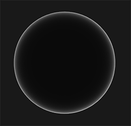
$$represents the base reflectivity of the surface, which we calculate using something called the refractive indices or IOR (indices of refraction), and, as you can see on the surface of the sphere, the closer the viewing direction is to the boundaries of the visible sphere (the angle between the viewing direction and the median vector reaches 90 degrees), the stronger the Fresnel effect and, therefore, the reflection:

There are several subtleties associated with the Fresnel equation. The first is that the Fresnel-Schlick approximation is valid only for dielectrics or non-metallic surfaces. For surfaces of conductors (metals), the calculation of the base reflectivity using refractive indices will be incorrect, and we need to use a different Fresnel equation for the conductors. Since this is inconvenient, we use pre-calculated values ​​for surfaces with a normal incidence ($$) (with an angle of 0 degrees, as if we were looking directly at the surface) and interpolate this value based on the viewing angle in accordance with the Fresnel-Schlick approximation, so that we can use the same equation for both metals and nonmetals .

The response of the surface during normal incidence or base reflectivity can be found in large databases like this . Some common values ​​listed below are taken from the notes for Nati Hoffman's course:

An interesting observation: for all dielectric surfaces, the base reflectivity never rises above 0.17, which is the exception rather than the rule, whereas for conductors the base reflectivity is much higher and (mostly) lies in the range from 0.5 to 1.0. In addition, for conductors or metal surfaces, the base reflectivity is tinted, therefore$$ presented as an RGB triplet (reflectivity with a normal incidence may vary depending on the wavelength).

These specific signs of metal surfaces compared to dielectric ones gave rise to something called a metallic workflow: when we create materials of surfaces with an additional parameter, known as metalness, which describes whether the surface is metal or not.

Theoretically, the metallicity of the surface takes only two values: it is either metal or not; the surface cannot be both. However, most render pipelines allow you to adjust the metallicity of the surface linearly between 0.0 and 1.0. This is mainly due to the lack of material in the texture of sufficient accuracy to create the surface, for example, with small particles of dust and sand, scratches on the metal surface. By changing the metallicity value around these small non-metallic particles and scratches, we get visually more pleasant results.

Precomputing $$for both dielectrics and metals, we can use the same Fresnel-Schlick approximation for both types of surfaces, but we need to tint the base reflectivity if we have a metallic surface. Usually we do it like this:

vec3 F0 = vec3(0.04);
F0 = mix(F0, surfaceColor.rgb, metalness);

We determined the base reflectivity, which is approximately the same for most dielectric surfaces. This is another approximation since$$averaged over most common dielectrics. The base reflectivity of 0.04 is retained for most dielectrics and gives physically plausible results without the need to specify an additional surface parameter. Therefore, depending on the type of surface, we either take the base reflectance of the dielectric, or assume that F0 is given by the color of the surface. Because metal surfaces absorb all the refracted light, they do not have diffuse reflections, and we can directly use the diffuse surface texture as the base reflectivity.

We translate the Fresnel-Schlick approximation into a code:

vec3 fresnelSchlick(float cosTheta, vec3 F0)
{
    return F0 + (1.0 - F0) * pow(1.0 - cosTheta, 5.0);
}

where cosTheta is the result of the scalar product between the surface normal vector and the direction of view.

Cook-Torrens reflection equation

Knowing all the components of the BRDF Cook-Torrens, we can include it in the final reflection equation:

$$

However, this equation is not completely mathematically correct. You probably remember that the Fresnel equation F is the coefficient of the amount of light reflected by a surface. That is actually our coefficient$$, which means that the mirror part of the reflection equation already contains $$. Given this, our final reflection equation is written as:

$$

This equation now fully describes the physical rendering model, which we usually call physically correct rendering or PBR. Do not worry if you have not fully understood how we need to arrange all the mathematics under discussion in the form of a code. In the following lessons we will look at how to use the reflection equation to get much more physically plausible results in our rendering, and all the pieces will be gathered together into a single unit.

Creating materials for PBR

Now, knowing the basic mathematical model of PBR, we end the discussion with a description of how artists usually define the physical properties of a surface, which we can directly transfer to the PBR equations. Each of the surface parameters we need for the PBR pipeline can be defined or modeled with textures. The use of textures gives us fragmentary control over how each specific point on the surface should react to light: is it metallic, rough or smooth, or how does this surface react to different wavelengths of light.

Below you will see a list of textures that can often be found in the PBR pipeline, as well as the result of their use:

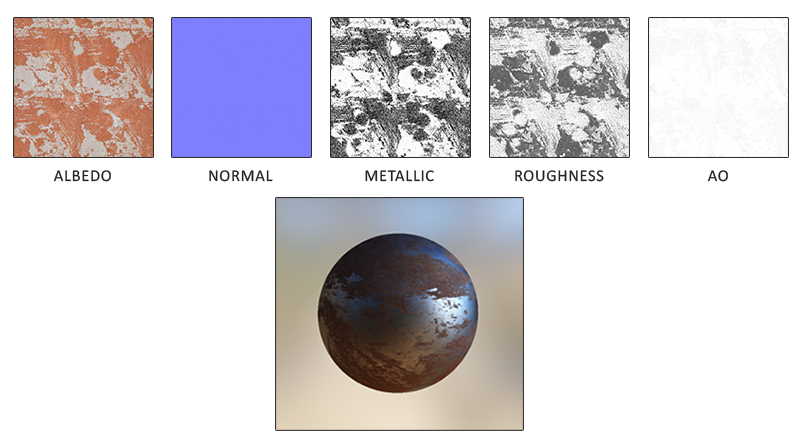
Albedo : The texture of the albedo determines for each texel the surface color or the base reflectivity, if this texel is metallic. This is a lot like the diffuse textures we used before, but all the lighting information is removed from the texture. Diffuse textures often have small shadows or darkened cracks inside the image, which is not necessary in the albedo texture; it should contain only the color of the surface.

Normals : the texture of the normal map is exactly the same as we used earlier in the tutorial on normal maps . The normal map allows us to set our normal for each fragment in order to create the illusion that the surface is more convex.

Metallicity : the metallicity map determines whether the texel is metallic or not. Depending on how the PBR engine is configured, artists can set metallicity in shades of gray or in two colors only: black and white.

Roughness : Roughness map indicates how rough the surface is at the heart of the texel. The roughness value selected from the texture determines the statistical orientation of the microfaces of the surface. On a rougher surface, broader and more diffuse reflections are obtained, while on a smooth surface they are focused and clear. Some PBR engines use smoothness maps instead of roughness maps, which some artists find more intuitive, but these values ​​translate into roughness (1.0 - smoothness) at the time of sampling.

AO (ambient occlusion) : Background shading maps or AO determine the additional shading factor of the surface and surrounding geometry. If we have a brick surface, for example, the albedo texture should not have any information about shading inside the brick gaps. The AO map defines these darkened faces, for which the light is more difficult to penetrate. Given the AO at the end of the lighting stage, we can significantly improve the visual quality of the scene. AO maps for meshes and surfaces are either generated manually or computed in 3D modeling programs.

Artists set and customize input values ​​for each texel and can base their textures on the physical properties of the surface of real materials. This is one of the biggest advantages of the PBR conveyor, since these physical properties of the surface remain unchanged from environmental conditions or lighting, which makes it easier for artists to obtain plausible results. Surfaces created in the PBR pipeline can be easily used in various PBR engines, and will look correct regardless of the environment in which they are located, which as a result looks much more natural.

Materials on the topic

• Background: Physics and Math of Shading by Naty Hoffmann: a lot of theory to fit in one article, so the theory hardly touches the basics here; If you want to learn more about the physics of light and how it relates to the PBR theory, this must-read resource is for you.
• Real shading in Unreal Engine 4 : A discussion of the PBR model adopted by Epic Games in the Unreal Engine 4. The PBR we are talking about in these tutorials is based on this model.
• Marmoset: PBR Theory : introduction to PBR. Mainly intended for artists, but nonetheless worth reading.
• Coding Labs: Physically based rendering : the basics of the rendering equation and how it relates to PBR.
• Coding Labs: Physically Based Rendering - Cook – Torrance : Cook-Torrens BRDF Fundamentals
• Wolfire Games - Physically based rendering : an introduction to PBR by Lukas Orsvärn.
• [SH17C] Physically Based Shading : an excellent interactive shadertoy (warning: it can take a long time to load) from Krzysztof Narkowi, demonstrates the interaction of light with PBR material.