Fourier in MP3 JPEG Wi-Fi: signal decomposition

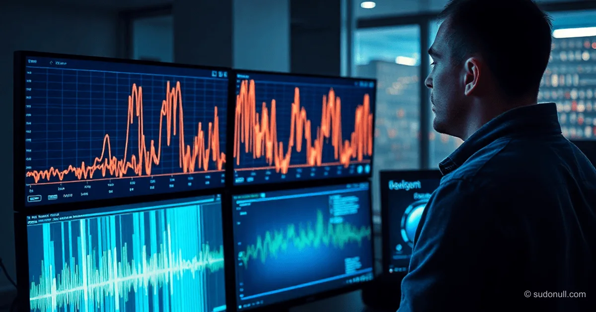
The Fourier Transform: The Foundation of MP3, JPEG, Wi-Fi, and MRI Compression

Any signal—from an audio track to a radio wave—can be broken down into a sum of sine waves with different frequencies, amplitudes, and phases. This is the idea from Jean-Baptiste Fourier in 1807, which Lagrange dismissed as impossible. The process is reversible and lossless.

Any signal = sin(f₁) × a₁ + sin(f₂) × a₂ + sin(f₃) × a₃ + ...
where f is frequency, a is amplitude

This decomposition is applied in audio processing, image handling, and wireless communication. FFT (Fast Fourier Transform) speeds up computations from O(n²) to O(n log n), making practical use possible.

MP3 Compression via Psychoacoustics and FFT

MP3 reduces the bitrate from 1.4 Mbps (CD) to 128 Kbps. The algorithm uses FFT to transition to the frequency domain.

# Pseudocode for MP3 compression
frequencies = fft(audio_signal)

for f in frequencies:
    if f.frequency > 20000:     # the ear can't hear above 20 kHz
        f.amplitude = 0
    if f.is_masked_by(louder_neighbor):  # psychoacoustic model
        f.amplitude = 0          # quiet sounds near loud ones are inaudible
    if f.amplitude < threshold:  # too quiet
        f.amplitude = 0

compressed = encode(remaining_frequencies)

Frequencies above 20 kHz and masked components are discarded. Decoding involves an inverse FFT. The difference is imperceptible to the human ear.

JPEG and DCT for Images

JPEG uses DCT (Discrete Cosine Transform)—a variant of Fourier—on 8×8 pixel blocks. Low frequencies preserve shapes, while high frequencies (details, noise) are quantized.

8×8 pixel block
    ↓
DCT: decomposition into "visual frequencies"
    ↓
Low frequencies = smooth gradients, general shapes
High frequencies = sharp edges, fine details, noise
    ↓
Discard high frequencies (the eye won't notice in a sunset photo)
    ↓
Compressed image, 10–20 times smaller than the original

Artifacts like blockiness result from excessive high-frequency cutoff. Inverse transformation restores the image.

OFDM in Wi-Fi and Mobile Communication

OFDM (Orthogonal Frequency-Division Multiplexing) modulates data onto hundreds of subcarrier frequencies within an 80 MHz wide channel. Subcarriers are orthogonal due to sine wave properties.

One Wi-Fi channel 80 MHz wide:

[subc.1][subc.2][subc.3]...[subc.234]
  ↓       ↓       ↓            ↓
 data    data    data    ...  data

All frequencies are transmitted SIMULTANEOUSLY.
The receiver separates them back via FFT.

Wi-Fi 6 uses 4096-QAM on 980 subcarriers. The receiver applies IFFT for demodulation. Similarly in 4G/5G, DSL, DVB-T.

• OFDM Advantages: resilience to multipath propagation, high spectral efficiency.
• Computations: FFT/IFFT in real-time on chips.
• Scale: billions of devices perform trillions of FFTs per second.

Recognition in Shazam and MRI

Shazam: FFT of audio → spectrogram → frequency peaks as fingerprints → database search.

1. Record 3 seconds of audio
2. FFT → spectrogram
3. Find peaks → fingerprints
4. Compare with database

Peaks are robust to noise. MRI: magnet resonates protons, records k-space (frequency domain). Inverse FFT yields an image.

Protons resonate → radio waves → k-space
     ↓
Inverse FFT
     ↓
Image

Implementing FFT in Python

Recursive FFT to understand the Cooley-Tukey algorithm.

import numpy as np

def fft(x):
    n = len(x)
    if n == 1:
        return x
    even = fft(x[0::2])
    odd = fft(x[1::2])
    T = [np.exp(-2j * np.pi * k / n) * odd[k] for k in range(n // 2)]
    return [even[k] + T[k] for k in range(n // 2)] + \
           [even[k] - T[k] for k in range(n // 2)]

Speedup enables real-time signal processing.

Key Takeaways

• Fourier decomposition is universal for wave processes: sound, light, radio waves.
• FFT reduces complexity from O(n²) to O(n log n), enabling quadrillions of operations per second.
• Applications: compression (MP3/JPEG), communication (OFDM), medicine (MRI), recognition (Shazam).
• Orthogonality of sine waves ensures signal separation without interference.
• The physics of the world is a sum of basic oscillations; Fourier decodes this language.

— Editorial Team