Machine Learning - 3. Poisson Random Process: Views and Clicks
- Tutorial
In previous articles on the probabilistic description of site conversion, we considered the number of events (views and clicks) as a sample of a random variable, regardless of time. Now it's time to take the next step and introduce it into consideration.
The random process f (t) is, slightly simplifying, a random variable that depends on time. The set of values of f (t) for a certain period of time T is called the implementation or selection of a random process. For example, the number of page views per day is an example of a discrete random process (or random sequence), for it both the argument (time) and the range of values, i.e. possible values of f (t) are discrete quantities. Accordingly, the sample of the random process will be the vector f (t i ). An example of two samples of random processes is shown in the graph (the calculations, like everything in my blog, were prepared using Mathcad Express and you can take them here ).
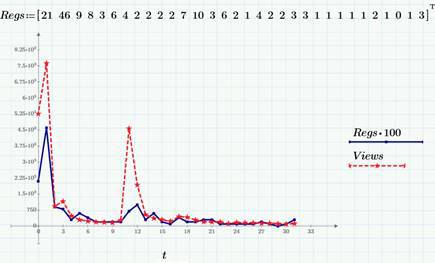
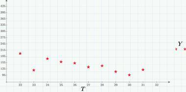
As examples, we still use the data on the views (Views row, red dotted line) and clicks (Regs, with a factor of 100) on this blog in Habré in March 2015, which we discussed in detail here and here . In particular, in the second article, we found out that a few days after the release of each article on Habr, the number of views and clicks reaches an approximately constant level of 100-200 views and 1-3 clicks per day, i.e. we can say that after a short period of non-stationarity, a random process can be considered stationary(neglecting, of course, a weak decreasing trend and a correction for dependence on the day of the week, which I hope to talk about in future articles when we get to detrending). The next graph is the stationary "tail" of the number of views (for the end of March 2015).
As we already see, random processes can be classified by the nature of the argument and values (whether they are discrete or continuous). It is easy to figure out that four combinations are possible (for more details, see, for example, Tikhonov’s book “Statistical Radio Engineering”). An example of a discrete process with continuous time is the number of times a site is viewed (or clicks on a site), starting at some point in time (for example, from the moment an article is published). The following graph shows an example of the implementation of such a process - the number of clicks during one of the days (March 22, 2015).

What can we say about the views / clicks model by looking at the latest graph? Obviously, we have two sequences of random events (event A - view and event B - click on some link) that can occur at random times. Accordingly, the random process b (t), the implementation of which is shown in the previous graph, is defined as the number of clicks starting from midnight on March 22 to time t.
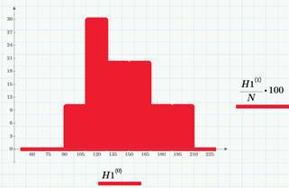
It is logical to assume that for any period of time (for example, an hour or a day) the probability of an event (A or B) to occur depends only on the duration of this period (this property is called uniformityrandom process in time). For example, if in an hour there are about 6 views of an article, then in a day there will be about 6 * 24 ~ 140. Or, if an average of 2 clicks occurs per day, then we can conditionally say that the average number of clicks per hour is 1/12. The histogram shows the variation in the number of views corresponding to the “tail”. Selected average values are λ = 140 views and λ2 = 1.2 clicks (per day).
It is important to make a few reservations here. Firstly, this approach is purely probabilistic in nature. We do not know in advance either the exact number of clicks per day, nor the moments at which the clicks will occur. Secondly, we still know something about the situation: that about 140 people open an article a day and 1-3 of them click in a certain place in the article. Thirdly, of course, the daily trend will be present in the data (during the day the article is read much more than at night). For simplicity (and for the time being - when we get to detrending), we will also neglect it. And, in the fourth (attention!), Until we talk about what the probability of events A and B is equal to (views and clicks).
As is known from the theory of probability formulated by a model called the random Poisson process or the Poisson stream of events , not only views and clicks are described well, but also a huge number of other real phenomena: phone calls, equipment failures (soon there will be a separate article about this here), requests for service, etc. If we agree to consider the sample function as continuous on the right, then, as shown in the corresponding figure above, it will be integer, and increasing only integer jumps. Accordingly, the probability density of the number of clicks and views will be discrete, as shown in the figure (for the case of clicks, a row in the form of red “sticks”):
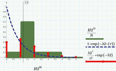
In the same figure, the “columns” (which is clear, but a little wrong, because we are talking about a discrete process) show the corresponding histogram of the distribution by the number of clicks, but we will talk about the meaning of the dashed curve a bit later. The formula for the Poisson probability density is given on the graph (in the "sticks" legend). Thus - attention! - calculating the sample average value of the number of clicks λ2 = 1.2 (click per day), we get a tool for forecasting, and, considering it together with conversion data (see previous articles), we get an algorithm for calculating the required number of visits to achieve certain target indicators for clicks.
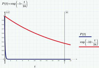
Another important quantity characterizing the Poisson process is the waiting time of the first event τ . Obviously, τIs a random variable. It is known from probability theory that its distribution function is exponential and is given by the formula F (t) = P ( τ
1-F (t) = exp (-λt). For clarity, we will draw this distribution function on the graph, choosing hours as the units of time (not a day). The blue P (t) curve refers to views, and the red to clicks.
Accordingly, the probability density of the waiting time is written as follows:

The distribution density of the number of views was denoted by the function p (t) in order to recall the relationship between the distribution density and the probability density of a random variable.
It is easy to calculate that the average value of the time for waiting for the first click is 1 / λ2, and for viewing, respectively, 1 / λ, which gives an idea of the simple probabilistic sense of the parameter λ as the average number of events occurring per unit time and equal to the average time to wait for the first event.
References:
Random processes
The random process f (t) is, slightly simplifying, a random variable that depends on time. The set of values of f (t) for a certain period of time T is called the implementation or selection of a random process. For example, the number of page views per day is an example of a discrete random process (or random sequence), for it both the argument (time) and the range of values, i.e. possible values of f (t) are discrete quantities. Accordingly, the sample of the random process will be the vector f (t i ). An example of two samples of random processes is shown in the graph (the calculations, like everything in my blog, were prepared using Mathcad Express and you can take them here ).
As examples, we still use the data on the views (Views row, red dotted line) and clicks (Regs, with a factor of 100) on this blog in Habré in March 2015, which we discussed in detail here and here . In particular, in the second article, we found out that a few days after the release of each article on Habr, the number of views and clicks reaches an approximately constant level of 100-200 views and 1-3 clicks per day, i.e. we can say that after a short period of non-stationarity, a random process can be considered stationary(neglecting, of course, a weak decreasing trend and a correction for dependence on the day of the week, which I hope to talk about in future articles when we get to detrending). The next graph is the stationary "tail" of the number of views (for the end of March 2015).
As we already see, random processes can be classified by the nature of the argument and values (whether they are discrete or continuous). It is easy to figure out that four combinations are possible (for more details, see, for example, Tikhonov’s book “Statistical Radio Engineering”). An example of a discrete process with continuous time is the number of times a site is viewed (or clicks on a site), starting at some point in time (for example, from the moment an article is published). The following graph shows an example of the implementation of such a process - the number of clicks during one of the days (March 22, 2015).
What can we say about the views / clicks model by looking at the latest graph? Obviously, we have two sequences of random events (event A - view and event B - click on some link) that can occur at random times. Accordingly, the random process b (t), the implementation of which is shown in the previous graph, is defined as the number of clicks starting from midnight on March 22 to time t.
It is logical to assume that for any period of time (for example, an hour or a day) the probability of an event (A or B) to occur depends only on the duration of this period (this property is called uniformityrandom process in time). For example, if in an hour there are about 6 views of an article, then in a day there will be about 6 * 24 ~ 140. Or, if an average of 2 clicks occurs per day, then we can conditionally say that the average number of clicks per hour is 1/12. The histogram shows the variation in the number of views corresponding to the “tail”. Selected average values are λ = 140 views and λ2 = 1.2 clicks (per day).
It is important to make a few reservations here. Firstly, this approach is purely probabilistic in nature. We do not know in advance either the exact number of clicks per day, nor the moments at which the clicks will occur. Secondly, we still know something about the situation: that about 140 people open an article a day and 1-3 of them click in a certain place in the article. Thirdly, of course, the daily trend will be present in the data (during the day the article is read much more than at night). For simplicity (and for the time being - when we get to detrending), we will also neglect it. And, in the fourth (attention!), Until we talk about what the probability of events A and B is equal to (views and clicks).
Poisson stream of events
As is known from the theory of probability formulated by a model called the random Poisson process or the Poisson stream of events , not only views and clicks are described well, but also a huge number of other real phenomena: phone calls, equipment failures (soon there will be a separate article about this here), requests for service, etc. If we agree to consider the sample function as continuous on the right, then, as shown in the corresponding figure above, it will be integer, and increasing only integer jumps. Accordingly, the probability density of the number of clicks and views will be discrete, as shown in the figure (for the case of clicks, a row in the form of red “sticks”):
In the same figure, the “columns” (which is clear, but a little wrong, because we are talking about a discrete process) show the corresponding histogram of the distribution by the number of clicks, but we will talk about the meaning of the dashed curve a bit later. The formula for the Poisson probability density is given on the graph (in the "sticks" legend). Thus - attention! - calculating the sample average value of the number of clicks λ2 = 1.2 (click per day), we get a tool for forecasting, and, considering it together with conversion data (see previous articles), we get an algorithm for calculating the required number of visits to achieve certain target indicators for clicks.
Another important quantity characterizing the Poisson process is the waiting time of the first event τ . Obviously, τIs a random variable. It is known from probability theory that its distribution function is exponential and is given by the formula F (t) = P ( τ

Accordingly, the probability density of the waiting time is written as follows:
The distribution density of the number of views was denoted by the function p (t) in order to recall the relationship between the distribution density and the probability density of a random variable.
It is easy to calculate that the average value of the time for waiting for the first click is 1 / λ2, and for viewing, respectively, 1 / λ, which gives an idea of the simple probabilistic sense of the parameter λ as the average number of events occurring per unit time and equal to the average time to wait for the first event.
References:
- Pytiev Yu.P., Shishmarev I.A.
The course of probability theory and mathematical statistics for physicists. M .: Moscow State University, 1983 - Tikhonov V.I. Statistical radio engineering M: "Soviet Radio", 1966
- D.V. Kiryanov, E.N. Kiryanova. Computational Physics. M: Polybook Multimedia, 2005. §5. Random processes and fields