Spectral analysis of signals
Not so long ago, comrade Makeman described how, using spectral analysis, it is possible to decompose a sound signal into its component notes. Let's abstract from the sound a bit and assume that we have some digitized signal, the spectral composition of which we want to determine, and quite accurately.
Under the cut is a brief overview of the method of extracting harmonics from an arbitrary signal using digital heterodyning, and a little special, Fourier magic.
So what we have.
File with samples of the digitized signal. It is known that a signal is the sum of sinusoids with their frequencies, amplitudes and initial phases, and possibly white noise.
What do we do.
Use spectral analysis to determine:
- the number of harmonics in the signal composition, and for each: amplitude, frequency (hereinafter in the context of the number of wavelengths per signal length), the initial phase;
- the presence / absence of white noise, and in the presence of its standard deviation (standard deviation);
- the presence / absence of a constant component of the signal;
- arrange all this in a pretty PDF report
with blackjack andillustrations.
We will solve this problem in Java.
Materiel
As I already said, the structure of the signal is known: it is the sum of sinusoids and some kind of noise component. It so happened that for the analysis of periodic signals in engineering practice, a powerful mathematical apparatus, commonly referred to as the "Fourier analysis" , is widely used . Let's briefly analyze what kind of animal it is.
A little special, Fourier magic
Not so long ago, in the 19th century, the French mathematician Jean-Baptiste Joseph Fourier showed that any function satisfying certain conditions (time continuity, periodicity, satisfying the Dirichlet conditions) can be expanded in a series, which later received its name - Fourier series .
In engineering practice, the expansion of periodic functions in a Fourier series is widely used, for example, in problems of circuit theory: the non-sinusoidal input action is decomposed into the sum of sinusoidal ones and the necessary parameters of the circuits are calculated, for example, by the superposition method.
There are several possible options for writing the coefficients of the Fourier series, we just need to know the essence.
Fourier series expansion allows one to expand a continuous function into the sum of other continuous functions. And in general, a series will have an infinite number of members.
A further refinement of the Fourier approach is the integral transformation of his own name. Fourier transform .
Unlike the Fourier series, the Fourier transform decomposes the function not in discrete frequencies (the set of frequencies of the Fourier series in which decomposition is, generally speaking, discrete), but in continuous.
Let's take a look at how the coefficients of the Fourier series are related to the result of the Fourier transform, called, in fact, the spectrum .
A small digression: the spectrum of the Fourier transform is, in the general case, a complex function that describescomplex amplitudes of the corresponding harmonics. That is, the values of the spectrum are complex numbers, whose modules are the amplitudes of the corresponding frequencies, and the arguments are the corresponding initial phases. In practice, the amplitude spectrum and the phase spectrum are considered separately.

Fig. 1. Correspondence of the Fourier series and Fourier transform on the example of the amplitude spectrum.
It is easy to see that the coefficients of the Fourier series are nothing more than the values of the Fourier transform at discrete time instants.
However, the Fourier transform maps a continuous in time, infinite function to another, continuous in frequency, infinite function - the spectrum. What if we do not have a function that is infinite in time, but only some discrete part recorded in time? The answer to this question is given by the further development of the Fourier transform - the discrete Fourier transform (DFT) .
The discrete Fourier transform is designed to solve the problem of the need for continuity and infinity in time of the signal. In fact, we believe that we cut out some part of the infinite signal, and for the rest of the time domain we consider this signal to be zero.
Mathematically, this means that having the studied function f (t) infinite in time, we multiply it by some window function w (t), which vanishes everywhere except for the time interval of interest to us.
If the "output" of the classical Fourier transform is a spectrum - a function, then the "output" of the discrete Fourier transform is a discrete spectrum. And the samples of the discrete signal are also fed to the input.
The remaining properties of the Fourier transform do not change: they can be read about in the relevant literature.
We only need to know about the Fourier transform of the sinusoidal signal, which we will try to find in our spectrum. In the general case, this is a pair of delta functions symmetric with respect to the zero frequency in the frequency domain.
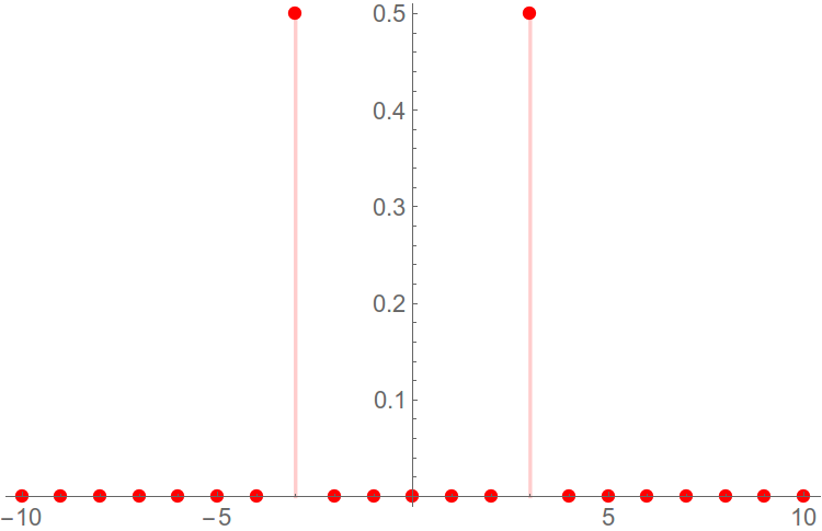
Fig. 2. The amplitude spectrum of the sinusoidal signal.
I have already mentioned that, generally speaking, we are not considering the original function, but some of its product with a window function. Then, if the spectrum of the original function is F (w) and the window is W (w), then the product spectrum will be such an unpleasant operation as the convolution of these two spectra (F * W) (w) (The convolution theorem).
In practice, this means that instead of a delta function, in the spectrum we will see something like this:
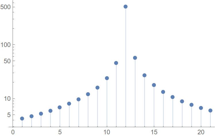
Fig. 3. The effect of spreading the spectrum.
This effect is also called spectral spreading (Eng. Spectral leekage). And the noises that appear due to spreading of the spectrum, respectively, by the side lobes (English sidelobes).
To combat side lobes, other, non-rectangular window functions are used. The main characteristic of the "efficiency" of the window function is the level of the side lobes (dB). A summary table of side lobe levels for some commonly used window functions is given below.
| Window function | Side lobe level (dB) |
| Dirichlet window (rectangular window) | -13 dB |
| Window hannah | -31.5 dB |
| Hamming Window | -42 dB |
The main problem in our problem is that the side lobes can mask other harmonics lying nearby.
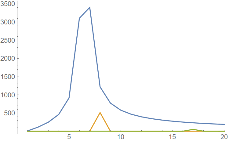
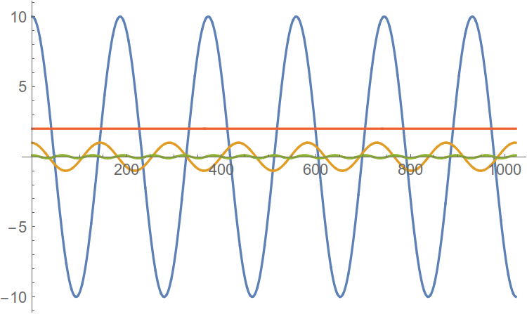
Fig. 4. Separate harmonic spectra.
It can be seen that, when the spectra are added together, the weaker harmonics dissolve in the stronger one.
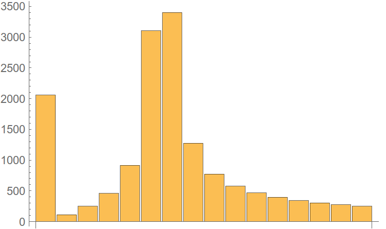
Fig. 5. Only one harmonic is clearly visible. Not good.
Another approach to controlling spreading of the spectrum is to subtract from the signal the harmonics that create this spreading.
That is, by setting the amplitude, frequency and initial phase of the harmonic, we can subtract it from the signal, and we will remove the “delta function” corresponding to it, and with it the side lobes generated by it. Another question is how exactly to know the parameters of the desired harmonic. It is not enough just to take the necessary data from the complex amplitude. The complex amplitudes of the spectrum are formed at integer frequencies, however, nothing prevents the harmonics from having a fractional frequency. In this case, the complex amplitude seems to be spread out between two adjacent frequencies, and its exact frequency, like other parameters, cannot be established.
To establish the exact frequency and complex amplitude of the desired harmonic, we will use a technique widely used in many branches of engineering practice - heterodyning .
Let's see what happens if we multiply the input signal by the complex harmonic Exp (I * w * t). The signal spectrum shifts w to the right.
We will use this property by shifting the spectrum of our signal to the right, until the harmonic becomes even more like a delta function (that is, until some local signal-to-noise ratio reaches a maximum). Then we can calculate the exact frequency of the desired harmonic, as w 0 - w get , and subtract it from the original signal to suppress the spreading effect of the spectrum.
An illustration of the change in spectrum depending on the local oscillator frequency is shown below.
Fig. 6. The type of amplitude spectrum depending on the frequency of the local oscillator.
We will repeat the described procedures until we cut out all the harmonics present and the spectrum will not remind us of the spectrum of white noise.
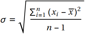
Then, it is necessary to evaluate the standard deviation of white noise. There are no tricks here: you can simply use the formula to calculate the standard deviation:
Automate it
It's time to automate the harmonics extraction. Let’s repeat the algorithm one more time:
1. We are looking for the global peak of the amplitude spectrum, above a certain threshold k.
1.1 If not found, finish
2. By varying the local oscillator frequency, we look for a frequency value at which a maximum of some local signal-to-noise ratio is reached in some vicinity of peak
3. If necessary, round off the values of the amplitude and phase.
4. Subtract the harmonic from the signal with the found frequency, amplitude and phase minus the local oscillator frequency.
5. We turn to step 1.
The algorithm is not complicated, and the only question that arises is - where do we get the threshold values above which we will look for harmonics?
To answer this question, it is necessary to evaluate the noise level even before cutting out the harmonics.
We will construct a distribution function (hi, math statistics), where the amplitude of harmonics will be on the abscissa axis, and the number of harmonics not exceeding the amplitude is the same value of the argument along the ordinate axis. An example of such a constructed function:
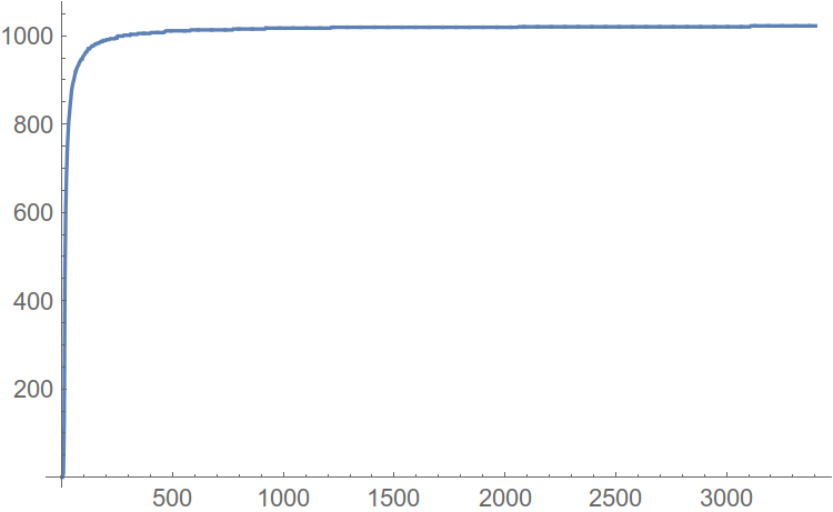
Fig. 7. Harmonic distribution function.
Now we also build a function - the distribution density. That is, the values of the finite differences of the distribution function.
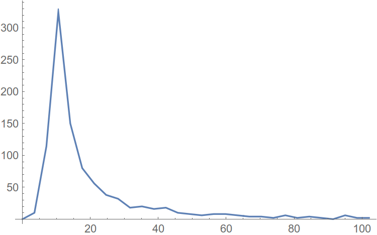
Fig. 8. The density of the harmonic distribution function.
The abscissa of the maximum of the distribution density is the amplitude of the harmonic that occurs in the spectrum the greatest number of times. We move away from the peak to the right by a certain distance, and we will consider the abscissa of this point to be an estimate of the noise level in our spectrum. Now you can automate.
Look at a piece of code that detects harmonics in a signal
public ArrayList detectHarmonics() {
    SignalCutter cutter = new SignalCutter(source, new Signal(source));
    SynthesizableComplexExponent heterodinParameter = new SynthesizableComplexExponent();
    heterodinParameter.setProperty("frequency", 0.0);
    Signal heterodin = new Signal(source.getLength());
    Signal heterodinedSignal = new Signal(cutter.getCurrentSignal());
    Spectrum spectrum = new Spectrum(heterodinedSignal);
    int harmonic;
    while ((harmonic = spectrum.detectStrongPeak(min)) != -1) {
        if (cutter.getCuttersCount() > 10)
            throw new RuntimeException("Unable to analyze signal! Try another parameters.");
        double heterodinSelected = 0.0;
        double signalToNoise = spectrum.getRealAmplitude(harmonic) / spectrum.getAverageAmplitudeIn(harmonic, windowSize);
        for (double heterodinFrequency = -0.5; heterodinFrequency < (0.5 + heterodinAccuracy); heterodinFrequency += heterodinAccuracy) {
            heterodinParameter.setProperty("frequency", heterodinFrequency);
            heterodinParameter.synthesizeIn(heterodin);
            heterodinedSignal.set(cutter.getCurrentSignal()).multiply(heterodin);
            spectrum.recalc();
            double newSignalToNoise = spectrum.getRealAmplitude(harmonic) / spectrum.getAverageAmplitudeIn(harmonic, windowSize);
            if (newSignalToNoise > signalToNoise) {
                signalToNoise = newSignalToNoise;
                heterodinSelected = heterodinFrequency;
            }
        }
        SynthesizableCosine parameter = new SynthesizableCosine();
        heterodinParameter.setProperty("frequency", heterodinSelected);
        heterodinParameter.synthesizeIn(heterodin);
        heterodinedSignal.set(cutter.getCurrentSignal()).multiply(heterodin);
        spectrum.recalc();
        parameter.setProperty("amplitude", MathHelper.adaptiveRound(spectrum.getRealAmplitude(harmonic)));
        parameter.setProperty("frequency", harmonic - heterodinSelected);
        parameter.setProperty("phase", MathHelper.round(spectrum.getPhase(harmonic), 1));
        cutter.addSignal(parameter);
        cutter.cutNext();
        heterodinedSignal.set(cutter.getCurrentSignal());
        spectrum.recalc();
    }
    return cutter.getSignalsParameters();
}
Practical part
I do not pretend to be a Java expert, and the solution presented may be questionable both in terms of performance and memory consumption, and in general the Java philosophy and OOP philosophy, no matter how hard I try to make it better. It was written in a couple of evenings, as proof of concept. Those interested can read the source code on GitHub .
The only difficulty was the generation of a PDF report based on the analysis results: PDFbox by no means wanted to work with the Cyrillic alphabet. By the way, he doesn’t want it now.
The following libraries were used in the project:
JFreeChart - displaying
PDFBox graphs - building a
JLatexMath report - rendering Latex formulas
As a result, we got a rather massive program (13.6 megabytes) that conveniently implements the task.
It is possible to cut harmonics manually, and entrust this task to the algorithm.
Thank you all for your attention!
An example of a report created by a program .
Literature
Sergienko A. B. - Digital Signal Processing