Fractal night
It was already the last hour of this Sunday, I was already thinking of going to bed, but a good sourcerer sent me a picture from my abandoned site, which can be seen below, and the text “beautiful!”. I painted these pictures about five years ago, using the so-called. runaway algorithm, but for the applicability of this algorithm, you need to be able to split the plane into regions for a given set of transformations, then I did not figure out how to do this, and did not return to this algorithm. But now I immediately figured out what to do and wrote to Dima: “First, Random IFS, then kNN, and then Escape-Time Algorithm!”
At hand I had only an old netbook, which my friends gave me for a while, while my laptop was being repaired. Dima still told me something, I answered something, but I already wrote code in my head, and I searched on the netbook for at least some compiler or interpreter and found C ++ Builder 6! After that, I realized that in the morning I would meet in private with the Borland compiler. Five hours later, I sent Dima new pictures, but he, as a normal person, had long slept ...
So, a little bit of formulas. Imagine that we have a finite set of transformations of the plane T i : R 2 → R 2 , i = 1, ..., k . For an arbitrary set E, we define T ( E ) = T 1 ( E ) ∪ ... ∪ T k ( E ), i.e., we act on each set on the set E , and combine the results. It can be proved that if the maps T i were contractive, then the sequence E , T ( E ),T ( T ( E )), ... converge to a plurality of F for all nonempty compact E . This construction is known as a system of iterable functions .
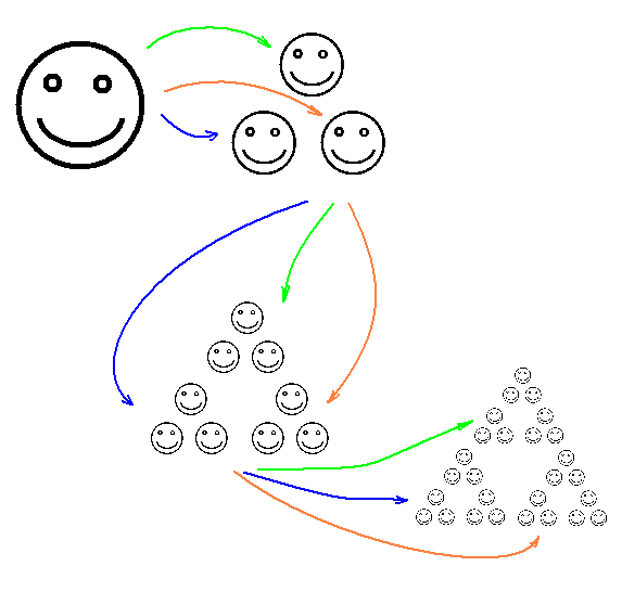
For example, if you take an emoticon as a non-empty compact set and consider three transformations, each of which is a compression and shift composition to the ith vertex of a regular triangle, then the first iterations will look like this, and in the limit we get the Sierpinski triangle:
Usually instead of directly calculating the sequence E , T ( E ), T ( T ( E)), ... for the construction of fractals use the so-called. "Game of chaos" , which is as follows. We choose an arbitrary point z 0 on the plane, then we randomly choose the transformation T i 1 and calculate z 1 = T i 1 ( z 0 ), then again randomly choose T i 2 and calculate z 1 = T i 2 ( z 0 ), and t etc. It can be shown that everything will be fine, and the set of points obtained will in some sense approximate the set Fdefined above. I will refer to this algorithm as Random IFS below.

Now is the time to move on to describing the runaway algorithm. Suppose we first have one transformation of the plane f . For each point z of the plane, we begin to calculate the sequence f ( z ), f ( f ( z )), f ( f ( f ( z ))), ... until either the number of iterations exceeds some given number N , or until the norm the number z becomes greater than a certain number of Bed and . After that, select the color of the point in accordance with the number of iterations performed.
If for a while we imagine that our plane is complex, and the transformation f ( z ) is equal to z 2 + c , then as a result of the operation of this algorithm we obtain a Julia fractal set . In more detail about it it is possible to read in habrastatj "Construction of Julia set" habraplusa mephistopheies .

Suppose now that we have a system of iterable functions defined by a set of reversible compressive transformations of the plane T 1 , ..., T k . Let F be an attractor of this system.
Additionally, suppose that the set Fcan be broken down so that T i ( F ) ∩ T j ( F ) = ∅, i ! = j (this assumption is far from always fulfilled). We divide the entire plane R 2 into pieces A 1 , ...., A k so that T i ( F ) is a subset of A i for all i . Now we define the function f ( z ) piecewise: on the set A i set f ( z ) =T k −1 ( z ) for all i .
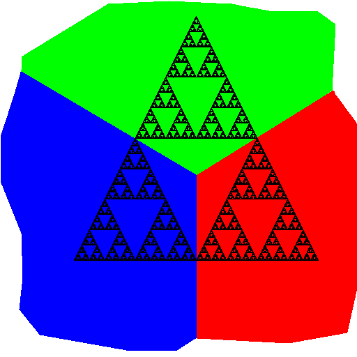
For example, for the Sierpinski triangle, we consider such a partition (there are minor problems with three points, but we close our eyes to them).
And now the main question is, what happens if the run-away time algorithm is applied to the function f constructed in this way ?
Let's see:

It turned out a pretty Sierpinski triangle!
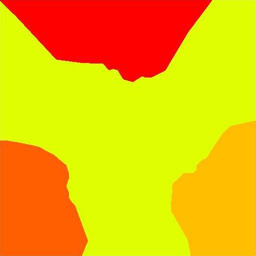
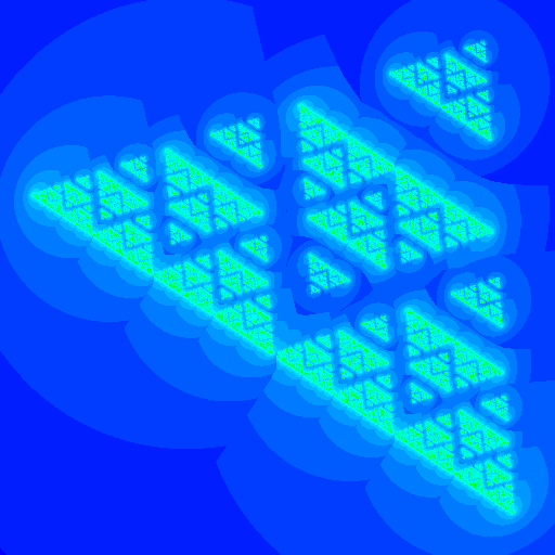
It turns out this is not an accident. A couple more examples:


In these examples, the corresponding plane partition is not difficult to determine analytically using Boolean combinations of circles and half-planes, using the method of close peering. But often simple conditions cannot be guessed. Therefore, instead of guessing, we will teach the computer to determine the partition on its own. The closest neighbor method will help us with this .
Namely, first with the help of Random IFS we generate several thousand points, while for each point we remember the transformation number with which it was obtained. Then, while running EscapeTimeAlgorithm for each pixel, we determine the area in which it falls using 1NN.
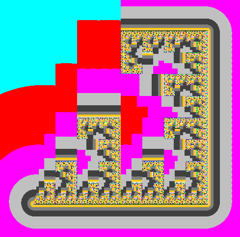
For example, for such an asterisk, 1NN gives the following splitting into four pieces: Putting it

together, we get:
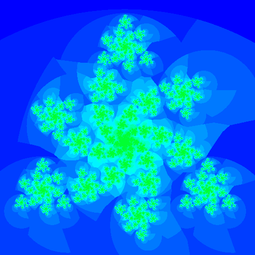
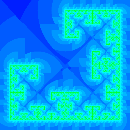
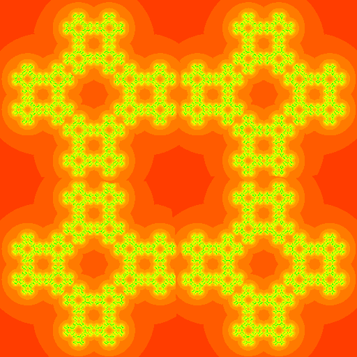
A few more pictures.

That's all. Finally, two comments.
Firstly, the attentive reader may have wondered if fractals that are built using Random IFS can be constructed using the run-time algorithm, is it possible to construct a Julia set using Random IFS? It turns out that you just need to reverse the map f ( z ) = z 2 + c , remembering how to extract the root from the complex number. (True, when applying this method to construct images of the Julia set, great difficulties arise.)

Secondly, the article described what happens, if you want to find out why this happens, I recommend M. Barnsley's book “Fractals Everywere”.
(Moments of source code can be found on the github .)

At hand I had only an old netbook, which my friends gave me for a while, while my laptop was being repaired. Dima still told me something, I answered something, but I already wrote code in my head, and I searched on the netbook for at least some compiler or interpreter and found C ++ Builder 6! After that, I realized that in the morning I would meet in private with the Borland compiler. Five hours later, I sent Dima new pictures, but he, as a normal person, had long slept ...


So, a little bit of formulas. Imagine that we have a finite set of transformations of the plane T i : R 2 → R 2 , i = 1, ..., k . For an arbitrary set E, we define T ( E ) = T 1 ( E ) ∪ ... ∪ T k ( E ), i.e., we act on each set on the set E , and combine the results. It can be proved that if the maps T i were contractive, then the sequence E , T ( E ),T ( T ( E )), ... converge to a plurality of F for all nonempty compact E . This construction is known as a system of iterable functions .
For example, if you take an emoticon as a non-empty compact set and consider three transformations, each of which is a compression and shift composition to the ith vertex of a regular triangle, then the first iterations will look like this, and in the limit we get the Sierpinski triangle:
Usually instead of directly calculating the sequence E , T ( E ), T ( T ( E)), ... for the construction of fractals use the so-called. "Game of chaos" , which is as follows. We choose an arbitrary point z 0 on the plane, then we randomly choose the transformation T i 1 and calculate z 1 = T i 1 ( z 0 ), then again randomly choose T i 2 and calculate z 1 = T i 2 ( z 0 ), and t etc. It can be shown that everything will be fine, and the set of points obtained will in some sense approximate the set Fdefined above. I will refer to this algorithm as Random IFS below.
z = (0, 0)
for (i = 0; i < maxIterNum; ++i) {
    cl = random([p1, ..., pk]) // pi -- вероятность, с которой выбираем преобразование Ti.
    z = T[cl](z)
    if (i > skipIterNum) { // Первых несколько итераций могут быть достаточно далеко от аттрактора.
        draw(z)
    }
}
Now is the time to move on to describing the runaway algorithm. Suppose we first have one transformation of the plane f . For each point z of the plane, we begin to calculate the sequence f ( z ), f ( f ( z )), f ( f ( f ( z ))), ... until either the number of iterations exceeds some given number N , or until the norm the number z becomes greater than a certain number of Bed and . After that, select the color of the point in accordance with the number of iterations performed.
for (y = y1; y < y2; y += dy) {
    for (x = x1; x < x2; x += dx) {
        z = (x, y);
        iter = 0;
        while (iter < N && ||z|| < B) {
             z = f(z)
             iter += 1;
        }
        drawPixel((x, y), color(iter))
    }
}
If for a while we imagine that our plane is complex, and the transformation f ( z ) is equal to z 2 + c , then as a result of the operation of this algorithm we obtain a Julia fractal set . In more detail about it it is possible to read in habrastatj "Construction of Julia set" habraplusa mephistopheies .

Suppose now that we have a system of iterable functions defined by a set of reversible compressive transformations of the plane T 1 , ..., T k . Let F be an attractor of this system.
Additionally, suppose that the set Fcan be broken down so that T i ( F ) ∩ T j ( F ) = ∅, i ! = j (this assumption is far from always fulfilled). We divide the entire plane R 2 into pieces A 1 , ...., A k so that T i ( F ) is a subset of A i for all i . Now we define the function f ( z ) piecewise: on the set A i set f ( z ) =T k −1 ( z ) for all i .
For example, for the Sierpinski triangle, we consider such a partition (there are minor problems with three points, but we close our eyes to them).

And now the main question is, what happens if the run-away time algorithm is applied to the function f constructed in this way ?
Let's see:

It turned out a pretty Sierpinski triangle!
It turns out this is not an accident. A couple more examples:


In these examples, the corresponding plane partition is not difficult to determine analytically using Boolean combinations of circles and half-planes, using the method of close peering. But often simple conditions cannot be guessed. Therefore, instead of guessing, we will teach the computer to determine the partition on its own. The closest neighbor method will help us with this .
Namely, first with the help of Random IFS we generate several thousand points, while for each point we remember the transformation number with which it was obtained. Then, while running EscapeTimeAlgorithm for each pixel, we determine the area in which it falls using 1NN.
For example, for such an asterisk, 1NN gives the following splitting into four pieces: Putting it


together, we get:
points = RandomIFS(Ts)
classifier = kNN(points);
for (y = y1; y < y2; y += dy) {
    for (x = x1; x < x2; x += dx) {
        z = (x, y)
        iter = 0
        while (iter < maxIterNum && ||z|| < sqrdBound) {
            cl = classifier.getClass(z);
            z = T[cl].applyInvert(z);
            iter += 1;
        }
        draw((x, y), color(iter))
    }
}
A few more pictures.


That's all. Finally, two comments.
Firstly, the attentive reader may have wondered if fractals that are built using Random IFS can be constructed using the run-time algorithm, is it possible to construct a Julia set using Random IFS? It turns out that you just need to reverse the map f ( z ) = z 2 + c , remembering how to extract the root from the complex number. (True, when applying this method to construct images of the Julia set, great difficulties arise.)
x = z0.re
y = z0.im
for (i = 0; i < N; ++i) {
    x -= c.re;
    y -= c.im;
    len = sqrt(x*x + y*y);
    ang = atan2(y, x);
    if (rand() % 2 == 0) { // Тут нужно что-нибудь и поинтереснее.
        x = sqrt(len) * cos(ang / 2);
        y = sqrt(len) * sin(ang / 2);
    } else {
        x = sqrt(len) * cos(ang / 2 + M_PI);
        y = sqrt(len) * sin(ang / 2 + M_PI);
    }
    draw(x, y)
}

Secondly, the article described what happens, if you want to find out why this happens, I recommend M. Barnsley's book “Fractals Everywere”.
(Moments of source code can be found on the github .)