A few words about “linear” regression

Sometimes this happens: the problem can be solved almost arithmetically, and first of all all Lebesgue integrals and Bessel functions come to mind. Here you start to train the neural network, then add a couple more hidden layers, experiment with the number of neurons, activation functions, then remember SVM and Random Forest and start all over again. And yet, despite the sheer abundance of entertaining statistical training methods, linear regression remains one of the popular tools. And for this there are preconditions, not the least among which is intuitiveness in the interpretation of the model.

Some formulas

In the simplest case, the linear model can be represented as follows:

y _i = a ₀ + a ₁ x _i + ε _i

where a ₀ is the mathematical expectation of the dependent variable y _i when the variable x _i is zero; a ₁ - the expected change in the dependent variable y _i when x _i changes by one (this coefficient is selected so that ½Σ (y _i - _{i i} ) ^{2 is} minimal - this is the so-called “residual function” ); ε _i is a random error.
In this case, the coefficients a ₁ and a ₀ can be expressed in terms of the Pearson correlation coefficient , standard deviations and average values ​​of the variables x and y:

â ₁ = cor (y, x) σ _y / σ _x

â ₀ = ȳ - â ₁ x̄

Diagnostics and model errors

For the model to be correct, it is necessary to fulfill the Gauss-Markov conditions , i.e. errors should be homoskedastic with zero expectation. The residual plot e _i = y _i - ŷ _i helps to determine how adequate the constructed model is (e _i can be considered an estimate of ε _i ).
Let us look at the graph of residuals in the case of a simple linear dependence y ₁ ~ x (hereinafter all examples are given in the language R ):


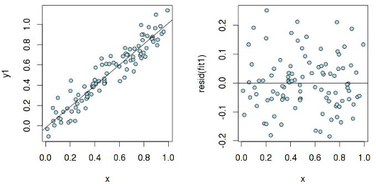
The residues are more or less evenly distributed relative to the horizontal axis, which indicates "the absence of a systematic relationship between the values ​​of the random term in any two observations." Now, let's examine the same graph, but built for a linear model, which is actually not linear:


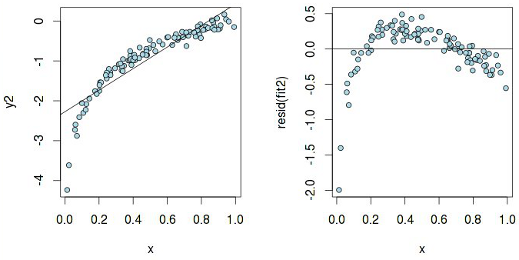
According to the graph y ₂ ~ x, it seems that a linear dependence can be assumed, but the residuals have a pattern, which means that pure linear regression will not work here . And here is what heteroskedasticity really means :


A linear model with such "swelling" residues is not correct. It is sometimes still useful to plot the quantiles of residues versus quantiles, which could be expected provided that the residues are normally distributed:


The second graph clearly shows that the assumption of the normality of the residues can be rejected (which again indicates the incorrectness of the model). And there are such situations:


This is the so-called "outlier" , which can greatly distort the results and lead to erroneous conclusions. R has a means to detect it - using the standardized measure dfbetas and hat values :

> round(dfbetas(fit4), 3)
    (Intercept)      x4
1        15.987 -26.342
2        -0.131   0.062
3        -0.049   0.017
4         0.083   0.000
5         0.023   0.037
6        -0.245   0.131
7         0.055   0.084
8         0.027   0.055
.....

> round(hatvalues(fit4), 3)
1     2     3     4     5     6     7     8     9     10...
0.810 0.012 0.011 0.010 0.013 0.014 0.013 0.014 0.010 0.010...

As can be seen, the first term of the vector x4 has a noticeably greater influence on the parameters of the regression model than the others, thus being an outlier.

Multiple Regression Model Selection

Naturally, with multiple regression the question arises: is it worth considering all the variables? On the one hand, it would seem that it costs, because any variable potentially carries useful information. In addition, increasing the number of variables, we increase R ² (by the way, for this reason, this measure cannot be considered reliable in assessing the quality of the model). On the other hand, it’s worth remembering things like AIC and BIC , which introduce penalties for the complexity of the model. The absolute value of the information criterion in itself does not make sense, therefore, it is necessary to compare these values ​​for several models: in our case, with a different number of variables. A model with a minimum value of the information criterion will be the best (although there is something to argue about).
Consider the UScrime dataset from the MASS library:

library(MASS)
data(UScrime)
stepAIC(lm(y~., data=UScrime))

The model with the lowest AIC value has the following parameters:

Call:
lm(formula = y ~ M + Ed + Po1 + M.F + U1 + U2 + Ineq + Prob, 
    data = UScrime)
Coefficients:
(Intercept)            M           Ed          Po1          M.F           U1           U2         Ineq         Prob  
  -6426.101        9.332       18.012       10.265        2.234       -6.087       18.735        6.133    -3796.032  

Thus, the optimal model taking into account AIC will be as follows:

fit_aic <- lm(y ~ M + Ed + Po1 + M.F + U1 + U2 + Ineq + Prob, data=UScrime)
summary(fit_aic)

...
Coefficients:
             Estimate Std. Error t value Pr(>|t|)    
(Intercept) -6426.101   1194.611  -5.379 4.04e-06 ***
M               9.332      3.350   2.786  0.00828 ** 
Ed             18.012      5.275   3.414  0.00153 ** 
Po1            10.265      1.552   6.613 8.26e-08 ***
M.F             2.234      1.360   1.642  0.10874    
U1             -6.087      3.339  -1.823  0.07622 .  
U2             18.735      7.248   2.585  0.01371 *  
Ineq            6.133      1.396   4.394 8.63e-05 ***
Prob        -3796.032   1490.646  -2.547  0.01505 *  
Signif. codes:  0 ‘***’ 0.001 ‘**’ 0.01 ‘*’ 0.05 ‘.’ 0.1 ‘ ’ 1

If you look closely, it turns out that the variables MF and U1 have a rather high p-value, which seems to hint to us that these variables are not so important. But p-value is a rather ambiguous measure when assessing the importance of a variable for a statistical model. This fact is clearly demonstrated by an example:

data <- read.table("http://www4.stat.ncsu.edu/~stefanski/NSF_Supported/Hidden_Images/orly_owl_files/orly_owl_Lin_9p_5_flat.txt")
fit <- lm(V1~. -1, data=data)
summary(fit)$coef

     Estimate Std. Error   t value     Pr(>|t|)
V2  1.1912939  0.1401286  8.501431 3.325404e-17
V3  0.9354776  0.1271192  7.359057 2.568432e-13
V4  0.9311644  0.1240912  7.503873 8.816818e-14
V5  1.1644978  0.1385375  8.405652 7.370156e-17
V6  1.0613459  0.1317248  8.057300 1.242584e-15
V7  1.0092041  0.1287784  7.836752 7.021785e-15
V8  0.9307010  0.1219609  7.631143 3.391212e-14
V9  0.8624487  0.1198499  7.196073 8.362082e-13
V10 0.9763194  0.0879140 11.105393 6.027585e-28

p-values ​​for each variable are almost zero, and we can assume that all variables are important for this linear model. But actually, if you look closely at the remnants, it somehow goes like this:


And yet, an alternative approach is based on analysis of variance , in which p-values ​​play a key role. Compare the model without the MF variable with the model built taking into account only AIС:

fit_aic0 <- update(fit_aic,  ~ . - M.F)
anova(fit_aic0, fit_aic)

Analysis of Variance Table
Model 1: y ~ M + Ed + Po1 + U1 + U2 + Ineq + Prob
Model 2: y ~ M + Ed + Po1 + M.F + U1 + U2 + Ineq + Prob
  Res.Df     RSS Df Sum of Sq      F Pr(>F)
1     39 1556227                           
2     38 1453068  1    103159 2.6978 0.1087

Given a P-value of 0.1087, with a significance level of α = 0.05, we can conclude that there is no statistically significant evidence in favor of an alternative hypothesis, i.e. in favor of a model with an additional variable MF

References:

1. Wonderful Regression Models Course
2. Residual Plots and Data Sets