Model of a natural series of numbers (nrch). Ulama spiral
The existing approaches to solving the problem of factorization of large numbers (HFBCH), intensively used in the world of mathematics for the last 20-30 years, indicate that for them this task is quite complicated, it stubbornly resists the external onslaught of specialists and does not give up positions. At the same time, I cannot mention works whose authors would offer a deep analysis of the problem, the state of the issue, or criticize the approach used. The basic principle in the approach is the sifting of many numbers (the sieve principle) dominates in this area, but it seems that this is not the only way and possibly not the best. Great hopes are placed on new types of computing devices, on new physical principles (quantum, molecular, etc.), but the change of approach is not discussed. Nevertheless, some conclusions already seem to be asking themselves today.
The RSA test number table published by RSA in 1991 is still far from complete. The published factorization results of part of the RSA numbers from this table allow us to conclude that the applied methods for solving the HFBCH are constructed using the properties of numbers that directly depend on the length (length) of the numbers. The shorter the number, the less time (in years) it took to factorize.
The second thing that attracts attention is an isolated, autonomous consideration of the factorizable number. The situation is now perceived so that the number N exists as if by itself, and is not selected from a well-organized, well-organized structure, its connections with the environment are broken, the properties inherent in the number do not inherit the properties of the environment and the location of the number in the environment.
A small example demonstrates the presence of such short-range bonds. For arbitrary three adjacent numbers, one of them is always a multiple of three, and the product of the extreme numbers is always equal to the square of the average number without unity,x = 24963 = 157 ∙ 159 . The position of the number 158 between 157 and 159 makes it easy to factor the number x.
In order to successfully overcome the crisis in the field of factorization theory, it is necessary to consider other approaches, in which the methods of solving the FBCH in which would be based on the properties of numbers that weakly depend or do not depend at all on the number capacity. These approaches are associated with the development of models of numerical systems as a whole and models of individual numbers within such systems.
Description of the NRF model and its features.Among the known models of the NRF spiral (Fig. 1), mathematician Stanislav Ulam (1909-1984) occupies a prominent place. It is remarkable for the simplicity of its structure and leaves an unforgettable impression of the first acquaintance with it and its perception. Essentially, a model is the cells of a plane digitized by numbers of a natural series, arranged in turns in the following order. In the middle of the paper sheet (see Fig. 2), 1 enters into the cell, 2 to the right of it, 3 to the top, 4 to the left, 6.7 to the left, 8.9 to the right, and the number 10, which begins a new spiral round. Each new round will call it a " circuit"increases its length by 8 cells in relation to the previous one. Further, as if continuing the tape with the width of the cell end-to-end, round-by-round, geometric squares are twisted counterclockwise - the model's contours. Each contour (square) will be supplied with serial number k, starting from the center of the spiral,k = 1,2,3, .... Cells with even and odd numbers are arranged in a spiral like cells on a chessboard. Diagonals of even and odd numbers alternate with each other.
Surprisingly, such a simple twisting of the linear list into a spiral introduces there is a strict order in the organization of numbers placed in the cells of the model. External signs of this order attract attention immediately, but what's inside ...?
Clarification of this issue and many others requires the availability of tools for working with elements and the object of the NRF as a whole. The aim of the proposed work is the preparation and creation of such tools.
The remarkable features of the model are, firstly, that the model is complete - all numbers of the natural series are displayed in spiral cells, and secondly, all cells containing numerical squares are aligned along one direction (along one line passing through the center), thirdly, all numerical squares are also divided into even squares on one side of the center, odd ones on the other; fourthly, vertical and horizontal rays, as well as odd diagonals, depart from the central contour k = 1, some of which are formed by cells in which prime numbers cannot be contained. The cells of these rays and diagonals go to infinity and contain only composite numbers.
S. Ulam himself noted with dark fill cells containing primes, and got a picture (Fig. 1) very similar from a space height to a multi-million city with its quarters and avenues. To some, the picture may even look like a starry sky, but the abundance of segments of straight lines and figures with right angles somewhat violates this similarity. When looking at the spiral, the conclusion suggests itself that there are not so few prime numbers, and their density per unit area, if it decreases with distance from the center, then the decrease is not visually felt
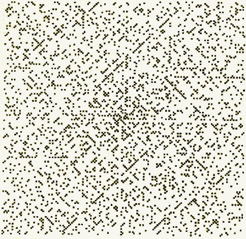
Figure 1 - Representation by a spiral of a fragment of a natural series with filled cells for primes ( 200x200 cells)
Various authors at different times made attempts to modify the appearance of the Ulam spiral. Zero was built into the center of the spiral; in particular, studies were carried out on a hexagonal numerical spiral. In addition, attempts were made to present a three-dimensional analogue of the Ulam spiral. So, for example, a numerical “spiral” was shown in the form of a flat triangle, along the height of which whole squares were lined up. The cone was illustrated as a result of “gluing together” the sides of a triangle having the same numerical values. Note that this way of presentation enhances the visibility, that is, it allows you to cover more numbers with a single glance than just on the number line. But in such works there are no means of studying, studying the model.
One of the goals of the author was the desire to use, to reveal the regularity of the appearance of
primes, to make it visual and convenient for further work with the model.
Introduction of a coordinate system . For practical work with the model and its elements, it is desirable to be able to select any single cell with two coordinates (x1, x2) or their group (contour), and establish in the cell with the given coordinates the numerical value N (x1, x2) assigned to it from the NRP, as functions of these coordinates. It is also desirable to be able to solve the inverse problem - given the given value N (x1, x2) of a natural number in an arbitrary cell, be able to determine its position in the model, i.e., its coordinates.
We show here how such problems are solved. The model as a whole is a discrete plane. With its clearly distinguishable elements (points, groups of points) we will consider individual cells and contours of cells, horizontal (G), vertical (B), diagonal (D) lines and rays .
Note that each circuit always contains a pair of cells filled with squares of different parity. We take for the beginning of the contour its cell with an odd square. This square will be called the left border of the kth contour - the smallest number in the contour. We denote the boundaries of the contour by the symbols Гл (k) = (2k - 1) ² - left (smaller) andГп (k) = (2k +1) ² - right (large).
Contour lengthL (k) will be called the number of cells in it. The length of the contour is calculated as L (k) = 8, k, or as the difference in the values of the odd squares - the boundaries of the contours starting with a pair of adjacent contours and is always a multiple of 8. This is easy to show, since it follows from the fact that the square of any odd number is 2n + 1 has the form1 + 8 ∙ Аi , where Аi is a combinatorial combination of two of n + 1. Therefore, for Аj> Аi, the square difference of two odd adjacent (and also not adjacent) numbers 1 + 8 ∙ Аj -1-8 8 Аi = 8 ∙ (Аj - Аi) is a multiple of 8. Semicircles are formed by dividing the contour into two parts: smaller m (k) with length L (m (k)) = Hz (k) -Gl (k) and larger M (k) with length L (M (k)) = Гп (k) -Hz (k) , where Hz (k) = (2k) ² - the common boundary of the half-circuits.
The lengths of all successive contours of the model form an infinitely increasing arithmetic progression with the difference d = 8 and the initial term a = 8.
The coordinate system of the model . For the origin we take the central cell with a unit. In the plane, the position of each point is uniquely described by two coordinates. Assignment of coordinates - localization of a point. It is convenient to perform such a localization of the point first with an accuracy to the contour, and then within the limits of a fixed contour - with the accuracy of the cell. Coordinates do not have to be Cartesian. With this approach, we assign the role of the first coordinate to the contour number (x1 = k). The role of the second coordinate x2, which determines the position of the cell in the circuit, is given to the distance (distance) of the cell from the beginning of the circuit.
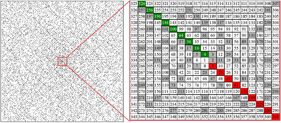
Figure 2 - The model of the NRF and an enlarged fragment of the central part of the spiral
In Figure 2, viewing a larger fragment of the NRF (399x399 cells), presented in a reduced form, makes it possible to verify that the expansion of the boundaries of the model does not substantially change the overall picture. From this figure, the central part with the number of cells 19x19 = 361 is cut out and the enlarged fragment with the number of cells filling is shown on the right. In the figure (with numbers), even in a limited volume, bands (highways) that do not contain filled cells are clearly visible.
This observation of highways leads to a definite conclusion regarding the prime numbers of twins. In each circuit, there are positions (cells) that cannot be occupied by primes and twins. For example, a pair of simple twins cannot be in the cells of the roadsides of the double highway, and these are four successive cells in a row and two of them are odd. Between twins (P> 7) there should always be a cell with an even number. The values of the four such numbers for any circuit are uniquely determined.
Example 1 . Let the number N = 39 be given. It is required to determine its position in the model, that is, (x1, x2) coordinates of the cell with this number.
Decision. We take the square root of the number N and round it to a smaller odd number. The value of the extracted square root is 6.244. The smallest nearest integer is 6 = 2k, the even number, the odd number smaller is 6 - 1 = 5. This number is odd and the cell containing its square 25 is the initial cell of the circuit containing the number N = 39. This is the smallest number (25) in the circuit . The square of the doubled contour number is equal to the only even square in the cells of the contour; it is obtained from the number per unit larger base of the odd square in the contour. Hence the contour number and the first coordinatex1 = k = 6/2 = 3 . An analysis of the situation shows that the number N = 39 is inscribed in the cell of the 3rd circuit (with the number k = 3) and this cell lies farther than an even square from the initial cell of this circuit. The second coordinate of the cell is found as the difference between the values of the given number N = 39 and the value of the odd square - the beginning of the contour, i.e. x2 = 39 - 25 = 14. The solution gets the form (x1, x2) = (3, 14) .
We solve the inverse problem. Let the cell (x1, x2) = (3, 14) be given by its coordinates. Find the number inscribed in the cell. The first coordinate is the contour number x1 = k = 3. The value of the number in the initial cell of the contour is found as an odd square, determined by the number k from the formula2k-1 = 2 ∙ 3 -1 = 5 . This square, obviously, is 25. The value of the number N in a given cell, remote from the initial cell of the circuit by x2 = 14, is determined by the sum N (x1, x2) = 25 + 14 = 39.
Thus, a method is proposed that provides selection (localization) of the NRF point specified by the number N on the planar model of the NRF, with two coordinates. And the solution of the inverse problem is to find its value by the given coordinates of the number N on the plane. A simple solution to these two problems allows you to perform data processing in a variety of tasks formulated with respect to the natural series of numbers. In subsequent posts, some of these tasks will be brought to the attention of readers.
Q = [λ] P
• ≠ ≢ ≡ ∄ ℕ ℤ ℝ ℙ ℒ ℂ ℚ ℍ ℘ ā ⊞ ∞ ∩ ∆ ℓ → ≤ ≥ & × Ø φ є ϵ ±
The RSA test number table published by RSA in 1991 is still far from complete. The published factorization results of part of the RSA numbers from this table allow us to conclude that the applied methods for solving the HFBCH are constructed using the properties of numbers that directly depend on the length (length) of the numbers. The shorter the number, the less time (in years) it took to factorize.
The second thing that attracts attention is an isolated, autonomous consideration of the factorizable number. The situation is now perceived so that the number N exists as if by itself, and is not selected from a well-organized, well-organized structure, its connections with the environment are broken, the properties inherent in the number do not inherit the properties of the environment and the location of the number in the environment.
A small example demonstrates the presence of such short-range bonds. For arbitrary three adjacent numbers, one of them is always a multiple of three, and the product of the extreme numbers is always equal to the square of the average number without unity,
In order to successfully overcome the crisis in the field of factorization theory, it is necessary to consider other approaches, in which the methods of solving the FBCH in which would be based on the properties of numbers that weakly depend or do not depend at all on the number capacity. These approaches are associated with the development of models of numerical systems as a whole and models of individual numbers within such systems.
Description of the NRF model and its features.Among the known models of the NRF spiral (Fig. 1), mathematician Stanislav Ulam (1909-1984) occupies a prominent place. It is remarkable for the simplicity of its structure and leaves an unforgettable impression of the first acquaintance with it and its perception. Essentially, a model is the cells of a plane digitized by numbers of a natural series, arranged in turns in the following order. In the middle of the paper sheet (see Fig. 2), 1 enters into the cell, 2 to the right of it, 3 to the top, 4 to the left, 6.7 to the left, 8.9 to the right, and the number 10, which begins a new spiral round. Each new round will call it a " circuit"increases its length by 8 cells in relation to the previous one. Further, as if continuing the tape with the width of the cell end-to-end, round-by-round, geometric squares are twisted counterclockwise - the model's contours. Each contour (square) will be supplied with serial number k, starting from the center of the spiral,
Surprisingly, such a simple twisting of the linear list into a spiral introduces there is a strict order in the organization of numbers placed in the cells of the model. External signs of this order attract attention immediately, but what's inside ...?
Clarification of this issue and many others requires the availability of tools for working with elements and the object of the NRF as a whole. The aim of the proposed work is the preparation and creation of such tools.
The remarkable features of the model are, firstly, that the model is complete - all numbers of the natural series are displayed in spiral cells, and secondly, all cells containing numerical squares are aligned along one direction (along one line passing through the center), thirdly, all numerical squares are also divided into even squares on one side of the center, odd ones on the other; fourthly, vertical and horizontal rays, as well as odd diagonals, depart from the central contour k = 1, some of which are formed by cells in which prime numbers cannot be contained. The cells of these rays and diagonals go to infinity and contain only composite numbers.
S. Ulam himself noted with dark fill cells containing primes, and got a picture (Fig. 1) very similar from a space height to a multi-million city with its quarters and avenues. To some, the picture may even look like a starry sky, but the abundance of segments of straight lines and figures with right angles somewhat violates this similarity. When looking at the spiral, the conclusion suggests itself that there are not so few prime numbers, and their density per unit area, if it decreases with distance from the center, then the decrease is not visually felt
Figure 1 - Representation by a spiral of a fragment of a natural series with filled cells for primes ( 200x200 cells)
Various authors at different times made attempts to modify the appearance of the Ulam spiral. Zero was built into the center of the spiral; in particular, studies were carried out on a hexagonal numerical spiral. In addition, attempts were made to present a three-dimensional analogue of the Ulam spiral. So, for example, a numerical “spiral” was shown in the form of a flat triangle, along the height of which whole squares were lined up. The cone was illustrated as a result of “gluing together” the sides of a triangle having the same numerical values. Note that this way of presentation enhances the visibility, that is, it allows you to cover more numbers with a single glance than just on the number line. But in such works there are no means of studying, studying the model.
One of the goals of the author was the desire to use, to reveal the regularity of the appearance of
primes, to make it visual and convenient for further work with the model.
Introduction of a coordinate system . For practical work with the model and its elements, it is desirable to be able to select any single cell with two coordinates (x1, x2) or their group (contour), and establish in the cell with the given coordinates the numerical value N (x1, x2) assigned to it from the NRP, as functions of these coordinates. It is also desirable to be able to solve the inverse problem - given the given value N (x1, x2) of a natural number in an arbitrary cell, be able to determine its position in the model, i.e., its coordinates.
We show here how such problems are solved. The model as a whole is a discrete plane. With its clearly distinguishable elements (points, groups of points) we will consider individual cells and contours of cells, horizontal (G), vertical (B), diagonal (D) lines and rays .
Note that each circuit always contains a pair of cells filled with squares of different parity. We take for the beginning of the contour its cell with an odd square. This square will be called the left border of the kth contour - the smallest number in the contour. We denote the boundaries of the contour by the symbols Гл (k) = (2k - 1) ² - left (smaller) and
Contour lengthL (k) will be called the number of cells in it. The length of the contour is calculated as L (k) = 8, k, or as the difference in the values of the odd squares - the boundaries of the contours starting with a pair of adjacent contours and is always a multiple of 8. This is easy to show, since it follows from the fact that the square of any odd number is 2n + 1 has the form
The lengths of all successive contours of the model form an infinitely increasing arithmetic progression with the difference d = 8 and the initial term a = 8.
The coordinate system of the model . For the origin we take the central cell with a unit. In the plane, the position of each point is uniquely described by two coordinates. Assignment of coordinates - localization of a point. It is convenient to perform such a localization of the point first with an accuracy to the contour, and then within the limits of a fixed contour - with the accuracy of the cell. Coordinates do not have to be Cartesian. With this approach, we assign the role of the first coordinate to the contour number (x1 = k). The role of the second coordinate x2, which determines the position of the cell in the circuit, is given to the distance (distance) of the cell from the beginning of the circuit.
Figure 2 - The model of the NRF and an enlarged fragment of the central part of the spiral
In Figure 2, viewing a larger fragment of the NRF (399x399 cells), presented in a reduced form, makes it possible to verify that the expansion of the boundaries of the model does not substantially change the overall picture. From this figure, the central part with the number of cells 19x19 = 361 is cut out and the enlarged fragment with the number of cells filling is shown on the right. In the figure (with numbers), even in a limited volume, bands (highways) that do not contain filled cells are clearly visible.
This observation of highways leads to a definite conclusion regarding the prime numbers of twins. In each circuit, there are positions (cells) that cannot be occupied by primes and twins. For example, a pair of simple twins cannot be in the cells of the roadsides of the double highway, and these are four successive cells in a row and two of them are odd. Between twins (P> 7) there should always be a cell with an even number. The values of the four such numbers for any circuit are uniquely determined.
Example 1 . Let the number N = 39 be given. It is required to determine its position in the model, that is, (x1, x2) coordinates of the cell with this number.
Decision. We take the square root of the number N and round it to a smaller odd number. The value of the extracted square root is 6.244. The smallest nearest integer is 6 = 2k, the even number, the odd number smaller is 6 - 1 = 5. This number is odd and the cell containing its square 25 is the initial cell of the circuit containing the number N = 39. This is the smallest number (25) in the circuit . The square of the doubled contour number is equal to the only even square in the cells of the contour; it is obtained from the number per unit larger base of the odd square in the contour. Hence the contour number and the first coordinate
We solve the inverse problem. Let the cell (x1, x2) = (3, 14) be given by its coordinates. Find the number inscribed in the cell. The first coordinate is the contour number x1 = k = 3. The value of the number in the initial cell of the contour is found as an odd square, determined by the number k from the formula
Thus, a method is proposed that provides selection (localization) of the NRF point specified by the number N on the planar model of the NRF, with two coordinates. And the solution of the inverse problem is to find its value by the given coordinates of the number N on the plane. A simple solution to these two problems allows you to perform data processing in a variety of tasks formulated with respect to the natural series of numbers. In subsequent posts, some of these tasks will be brought to the attention of readers.
• ≠ ≢ ≡ ∄ ℕ ℤ ℝ ℙ ℒ ℂ ℚ ℍ ℘ ā ⊞ ∞ ∩ ∆ ℓ → ≤ ≥ & × Ø φ є ϵ ±