Quaternion Encryption Scheme (QES) on FPGA, XeonPhi, GPU

Hi, Habrahabr!
Quaternion data was encrypted using FPGA DE5-NET, XeonPhi 7120P, and Tesla k20 GPU.
All three have approximately the same peak performance, but there is a difference in power consumption.
In order not to pile up the article with unnecessary information, I suggest you familiarize yourself with a brief information about what a quaternion and a rotation matrix are in the corresponding Wikipedia articles.
To find out the cryptographic strength of the QES algorithm, I ask you to use search engines for a detailed description of the algorithm, one of the authors of which is Nagase T., and one of the articles, for example, Secure signals transmission based on quaternion encryption scheme.
How can you encrypt and decrypt data using quaternions? Pretty simple!
First, take the quaternion: q = w + x * i + y * j + z * k and compose the rotation matrix on its basis, which we will call, for example, P (q).
Note the picture below is from Wikipedia and the matrix is named Q.
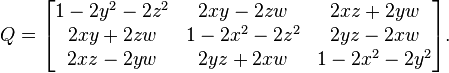
To encrypt data, you need to perform the usual matrix multiplication, for example: B ' = P (q) * B, where B is the data that needs to be encrypted, P (q) is the rotation matrix, B' is encrypted data.
To decrypt the data, as you probably already guessed, you need to multiply the “encrypted” matrix B 'by the inverse matrix (P (q)) ^ - 1, so we get the original data: B = (P (q)) ^ - 1 * B ' .
Source data matrices are filled on the basis of files or, as shown at the beginning, images.
Below is a variant of OpenCL code for FPGA, the need to transfer the encryption matrix in separate numbers is a necessity due to the features of the board.
__kernel void quat(__global uchar* arrD, uchar m1x0, uchar m1x1, uchar m1x2, uchar m1x3, uchar m1x4, uchar m1x5, uchar m1x6, uchar m1x7, uchar m1x8)
{
uchar matrix1[9];
matrix1[0] = m1x0;
matrix1[1] = m1x1;
matrix1[2] = m1x2;
matrix1[3] = m1x3;
matrix1[4] = m1x4;
matrix1[5] = m1x5;
matrix1[6] = m1x6;
matrix1[7] = m1x7;
matrix1[8] = m1x8;
int iGID = 3*get_global_id(0);
uchar buf1[3];
uchar buf2[3];
buf2[0] = arrD[iGID];
buf2[1] = arrD[iGID + 1];
buf2[2] = arrD[iGID + 2];
buf1[0] = matrix1[0] * buf2[0] + matrix1[1] * buf2[1] + matrix1[2] * buf2[2];
buf1[1] = matrix1[3] * buf2[0] + matrix1[4] * buf2[1] + matrix1[5] * buf2[2];
buf1[2] = matrix1[6] * buf2[0] + matrix1[7] * buf2[1] + matrix1[8] * buf2[2];
arrD[iGID] = buf1[0];
arrD[iGID+1] = buf1[1];
arrD[iGID+2] = buf1[2];
}
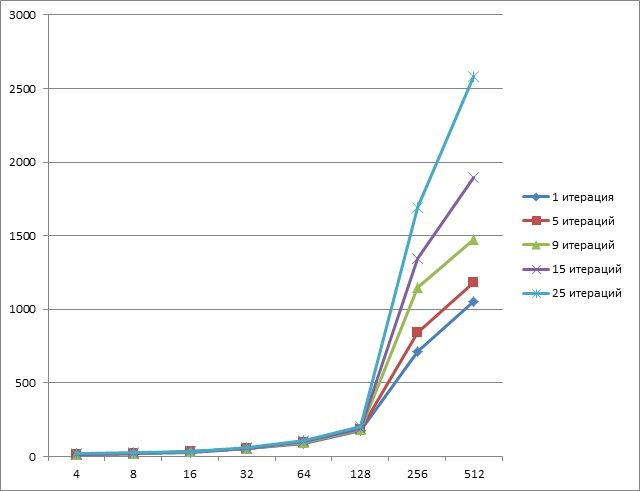
When using XeonPhi, the results were as follows (Y axis - time, ms; X axis - amount of data, Mb):

As you can see from the graph, XeonPhi responds well to the complexity of the task, that is, when using a conventional desktop processor, the time between 1 and 25 iterations differs approximately 25 times, while here about twice.
Unfortunately, these results are far from the best, because when programming, OpenMP technology and the ability to automatically optimize the Intel compiler were used. When programming at a lower level, i.e. for example intrinsic teams, results can improve several times.
When using Tesla k20, the results were as follows (Y axis - time, ms; X axis - amount of data, Mb):
As you can see, pipelining with a small data size shows itself perfectly.
When using the De5-Net FPGA, the results were as follows (Y axis - time, ms; X axis - amount of data, Mb):

At first glance, it seems that there is an error in the graph, but in fact, due to its architecture, FPGA shows an excellent level of pipelining regardless on the size of the data.
Thank you for your attention to this article.
UPD
Before reading all the comments, I recommend reading
habrahabr.ru/post/226779/#comment_7699309
This will save you a little time, thanks.