Determining the color of cars using neural networks and TensorFlow
Hello, my name is Roman Lapin, I am a 2nd year postgraduate student at the Faculty of the Higher School of General and Applied Physics at UNN. This year I managed to qualify and participate in the work of the Intel Summer School in Nizhny Novgorod. I was assigned the task of determining the color of a car using the Tensorflow library, on which I worked together with my mentor and engineer of the ICV team Alexey Sydnev.
And that's what I did.
There are several aspects to this task:
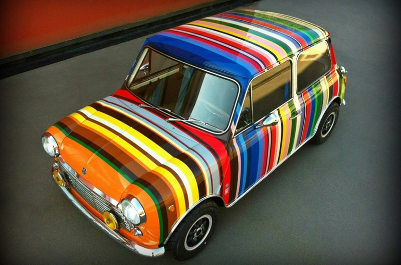
- The car can be painted in several colors, as in the KDPV. And in one of our datasets, for example, there was a car with camouflage colors.
- Depending on the lighting and the camera that captures what is happening on the road, cars of the same color will look very different. The “illuminated” cars may have a very small part that corresponds to the “true” color of the car.
Vehicle color detection
The color of the car is a rather strange substance. The manufacturer has a clear understanding of what color the car they produce, for example: phantom, glacial, black pearl, pluton, lime, krypton, angkor, carnelian, platinum, blues. The traffic police opinion about the colors of cars is quite conservative and very limited. Each individual person has a subjective perception of color (you can recall the popular story about the color of the dress). Thus, we decided to perform the markup as follows.
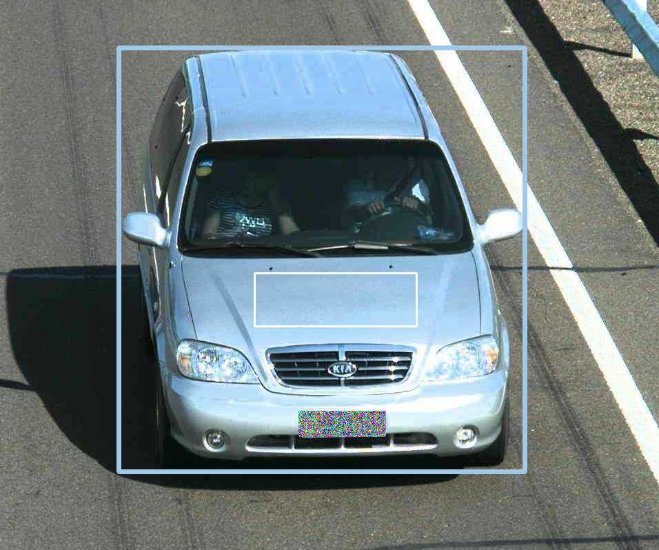
On each image, the coordinates of the vertices of the bordering rectangles around the cars were marked (hereinafter I will use the English version - car bounding box ) and inside them are the areas that best characterize the color of the vehicles ( color box). The number of the latter is equal to the color of the car ( n x color box - n-color car).
Hereinafter, the numbers of cars are smeared for the ability to publish photos in the public domain.
Dataset car layout
In the future, we worked with two color spaces - RGB and LAB - with 8 and 810/81 classes, respectively. To compare the results of different approaches, we used to determine the color of 8 classes in RGB, which are obtained by dividing the BGR cube into 8 equal small cubes. They can easily be called common names: white, black, red, green, blue, pink, yellow, cyan. To estimate the error of any method, we have already used the color space LAB, in which the distance between the colors is determined .
There are two intuitive ways to determine color by color box : medium or median color. But in the color boxThere are pixels of various colors, so I wanted to know how accurately each of these two approaches worked.
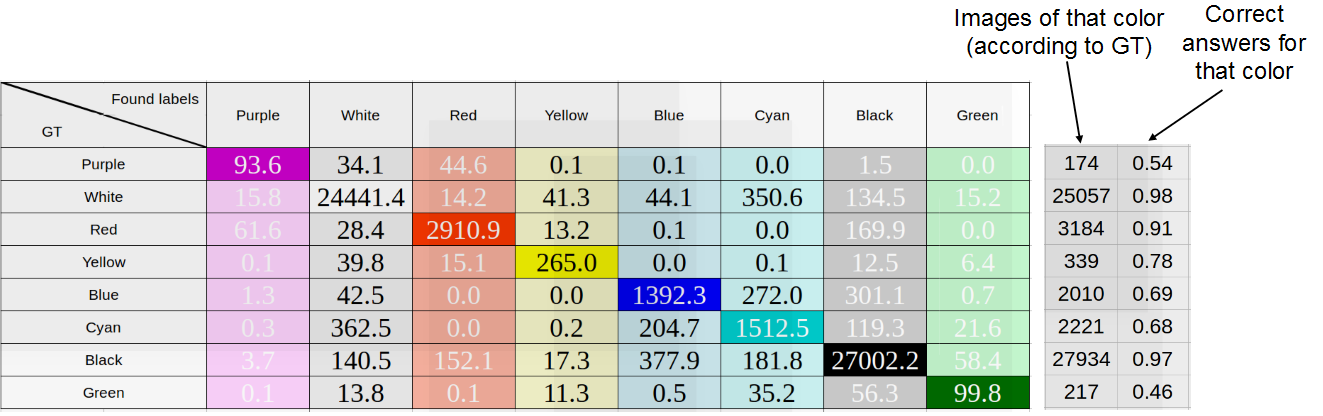
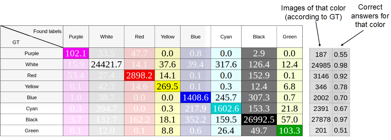
For 8 RGB colors for each color box of each machine in dataset, we determined the average color of pixels and the median, the results are shown in the figures below. “True” colors are marked in the rows — that is, colors defined respectively as medium or median, and in columns the colors occurring in principle. When adding one car to the table, the number of pixels of each color was normalized by their number, i.e. the sum of all values added to the line was equal to one.
The study of the accuracy of determining the color of the machine as the average color of pixels color 'abox. Average accuracy: 75%
The study of the accuracy of determining the color of the machine as the median color of the pixels color box. Average accuracy: 76%
As you can see, there is not much difference between the methods, which indicates good marking. Later we used the median, since it showed the best result.
The vehicle color determination will be based on the area inside the car bounding box .
Do we need networks?
The inevitable question is: do we really need neural networks to solve an intuitively simple task? Maybe you can take the median or average pixel color of the car bounding box in the same way ? The figures below show the result of this approach. As will be shown later, it is worse than the method using neural networks.

The distribution of the share of cars with the value of L2 error in the space LAB between the color box color, defined as the average, and the car bounding box color of the value of this error
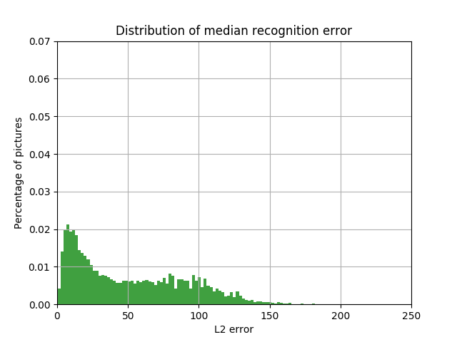
The distribution of the share of cars with the value of L2 errors in the LAB space between the color box color defined as the median and the car bounding box color of the value of this error
Description of the approach to the task
In our work, we used the Resnet-10 architecture to highlight features. To solve one label and multilabel tasks, the activation functions of softmax and sigmoid, respectively, were chosen .
An important issue was the choice of a metric by which we could compare our results. In the case of one label task, you can select the class corresponding to the maximum response . However, this solution will obviously not work in the case of multilabel / multi-color machines, since argmax produces one, most likely, color. The L1 metric depends on the number of classes, so it could not be used to compare all the results either. Therefore, it was decided to dwell on the metric of the area under the ROC curve(ROC AUC - area under curve) as universal and generally accepted.
We worked in two color spaces. The first is the standard RGB , in which we chose 8 classes: we broke the RGB cube into 8 identical sub-cubic pins: white, black, red, green, blue, pink, yellow, cyan. Such a partition is very rough, but simple.
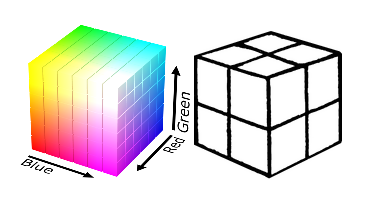
Splitting the RGB color space into 8 regions.
In addition, we conducted research with the color space LAB, which used a partition into 810 classes. Why so much? LAB was introduced after the American scientist David MacAdam established that there are areas of colors that are not distinguishable by the human eye ( Macadam ellipses ). LAB was constructed so that in it these ellipses had the form of circles (in the section of constant L - brightness).
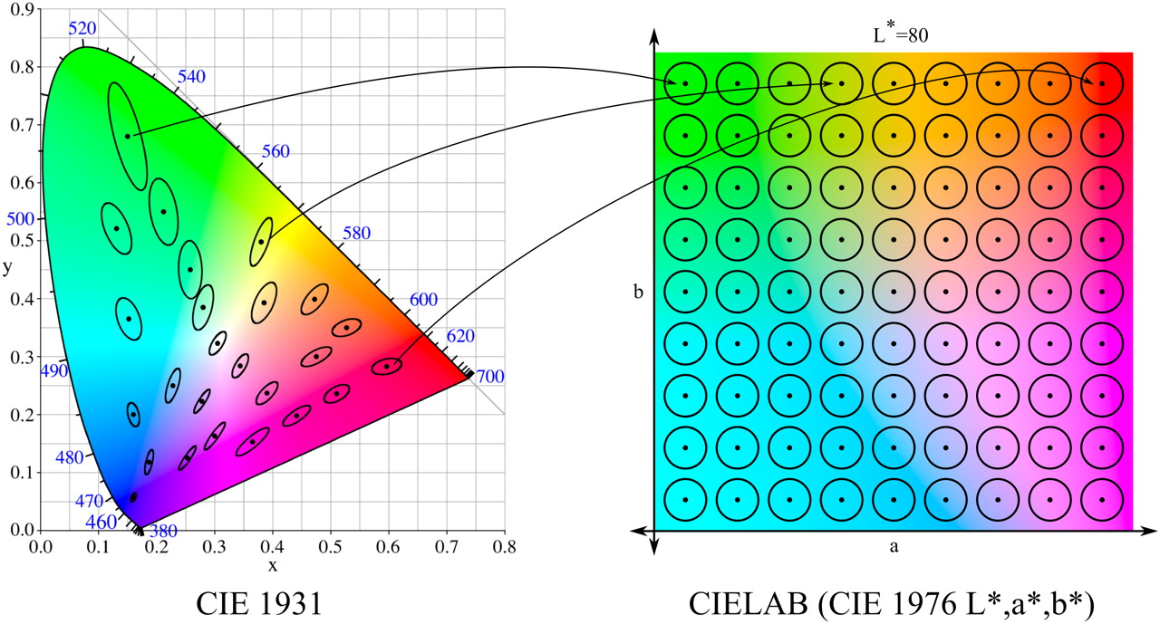
Macadam ellipses and color space LAB ( image source ).
In total, there are 81 such circles in the cross section. We took step 10 in the L parameter (from 0 to 100), receiving 810 classes. In addition, we conducted an experiment with a constant L and, accordingly, 81 classes.
RGB and LAB
For the 8-class problem and the RGB space, the following results were obtained:
| Activation function | Multilabel task | ROC AUC |
|---|---|---|
| softmax | - | 0.97 |
| sigmoid | ✓ | 0.88 |
It seems that the result for the multilabel task is already quite good. To test this assumption, we constructed an error matrix, taking the threshold for the probability of 0.55. Those. If this value is exceeded in probability for the corresponding color, we consider that the car is painted in this color too. Despite the fact that the threshold is chosen low enough, when it is possible to see the characteristic errors in determining the color of the car and draw conclusions.
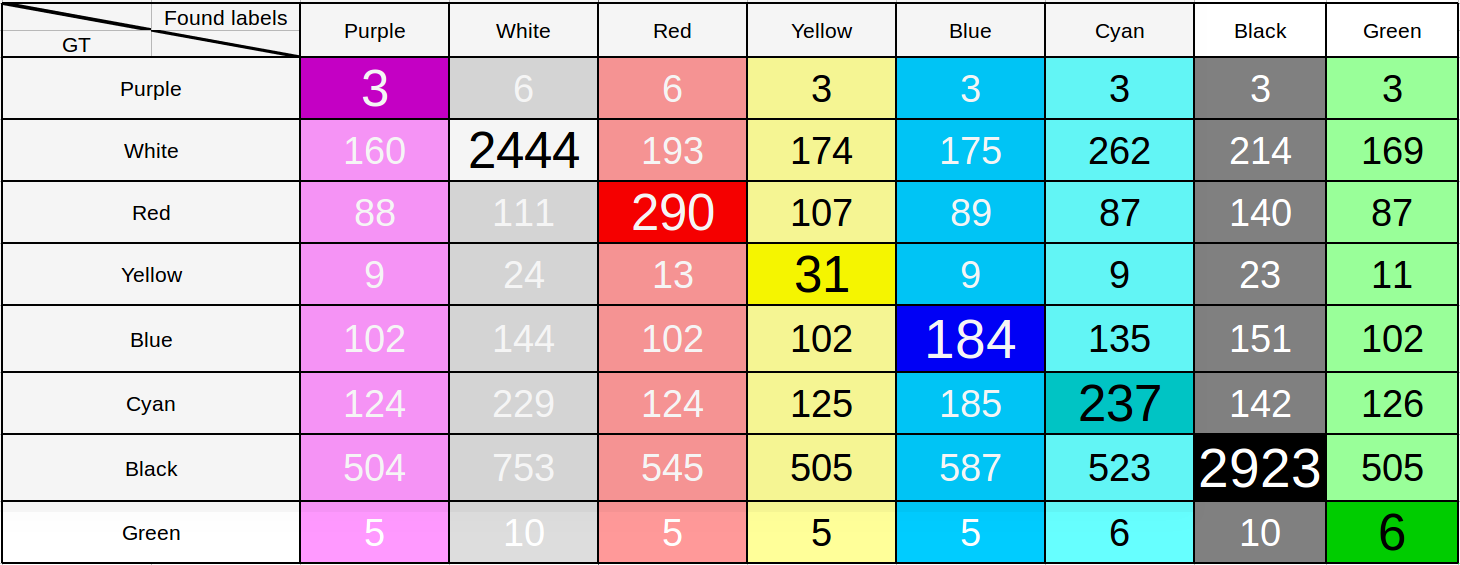
The table of results of recognition of the color of machines in the 8th class problem.
It is enough to look at the lines corresponding to the green or pink colors to make sure that the model is far from perfect. To the question of why, with a large value for the metric, we get such a strange unfortunate result, we will come back, let us immediately indicate: when considering only 8 classes, a huge number of colors fall into the “white” and “black” classes, therefore such an outcome .
Therefore, we next proceed to the color space LAB and conduct research there.
| Activation func | Multilabel task | ROC AUC |
|---|---|---|
| softmax | - | 0.915 |
| sigmoid | ✓ | 0.846 |
The result was smaller, which is logical, as the number of classes increased by two orders of magnitude. Taking the sigmoid result as a starting point, we tried to improve our model.
LAB: experiments with different weights
Before that, all experiments were performed with unit weights as a function of loss ( loss ):
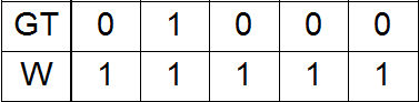
Here GT is ground truth, W is weights.
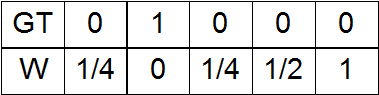
In the color space LAB you can enter the distance . Suppose we have one unit in GT. Then it corresponds to some rectangular parallelepiped in the color space LAB. This parallelepiped (more precisely, its center) is removed at a different distance from all other parallelepipeds (again, their centers). Depending on this distance, you can experiment with the following options for the scales:
a) Zero at the place of the unit in the GT, and as it moves away from it, an increase in the scale;
b) On the contrary, at the place of the unit in GT there is a unit; when removed, the scale decreases;

c) Option a) plus a small Gaussian additive with an amplitude of ½ at the site of the unit in the GT;
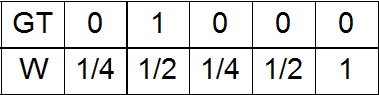
d) Option a) plus a small Gaussian additive with amplitude 1 in place of the unit in the GT;

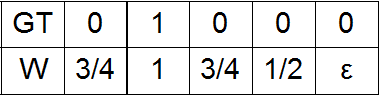
e) Option b) with a small addition at the maximum distance from one in GT.
The last version of the scales with which we conducted experiments was, as we called it, triple gauss, namely, three normal distributions with centers in place of units in the GT, as well as at the greatest distance from them.
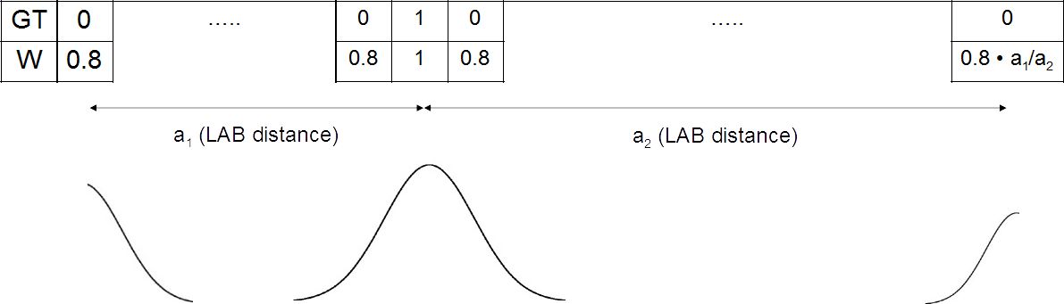
Three normal distributions with centers in place of units in the GT and with the greatest distance from them.
He will have to be explained in a little more detail. You can select the two most distant parallelepipeds, and, therefore, the class, and compare them by distance from the source. For the class corresponding to the far one, the amplitude of the distribution is set to 0.8, and for the second one is m times smaller, where m is the ratio of the distance from the source to the far distance to the distance between the source and neighbor.
The results are shown in the table. Due to the fact that in the scales of option a) there were zero weights - just units in GT, the result for them came out even worse than the starting point, since the network did not take into account successful color definitions, learning less. The weights b) and e) practically coincided, and therefore the result for them coincided. The largest increase in percentage points compared with the starting result was shown by the variant of weights f) - triple gauss.
| Activation function | Number of classes | Weights type | ROC AUC |
|---|---|---|---|
| sigmoid | 810 | a) | 0.844 |
| b), e) | 0.848 | ||
| c) | 0.888 | ||
| d) | 0.879 | ||
| f) | 0.909 |
LAB: experimenting with new labels
So, we conducted experiments with different weights in loss . Then we decided to try to leave the weights as single ones, and change the labels that are transferred to the loss function and are used to optimize the network. If before that labels coincided with GT, now they decided to use again Gaussian distributions with centers in place of units in GT:
The motivation for such a decision is as follows. The fact is that with ordinary labels all cars in datasets fall into a fixed number of classes, less than 810, so the network learns to determine the color of cars of only these classes. With new labels, non-zero values fall into all classes and we can expect an increase in the accuracy of determining the color of the car. We experimented with two sigmas (standard deviations) for the above Gaussian distributions: 41.9 and 20.9. Why such? The first sigma is chosen as follows: the minimum distance between the classes (28) is taken and sigma is determined from the condition of the distribution falling twice in the class next to the GT. And the second sigma is just less than the first two times.
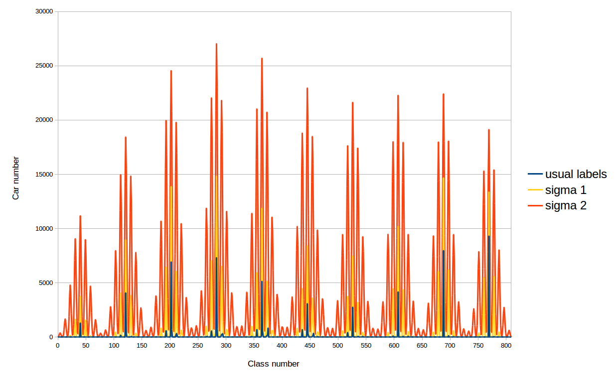
The distribution of training dataset cars by classes with different labels at loss
And indeed, it was possible to further improve the result with the help of such a trick, as shown in the table. As a result, the determination accuracy reached 0.955!
| Activation function | Number of classes | Labels type | Weights type | ROC AUC |
|---|---|---|---|---|
| sigmoid | 810 | usual | ones | 0.846 |
| usual | three gauss | 0.909 | ||
| new, σ 1 | three gauss | 0.955 | ||
| new, σ 2 | 0.946 |
LAB: 81
If we talk about unsuccessful experiments, it is necessary to mention an attempt to train the network with 81 classes and the constant parameter L. We observed in previous experiments that the brightness is determined quite accurately by the network, and we decided to practice only parameters a and b (so two other coordinates are called in LAB). Unfortunately, despite the fact that the network was able to train perfectly in the plane, showing a greater value in the metric, the idea of setting the L parameter at the output of the network as the average for the car bounding box failed and the actual color and thus determined differed very much.
Comparison with problem solving without using neural networks
And now let's go back to the very beginning and compare what we have, with recognizing the color of the car without using neural networks.
The results are shown in the figures below. It can be seen that the peak has become more than 3 times, and the number of cars with a large error between the true and a certain color has decreased significantly.
The distribution of the share of cars with the L2 value of the error in the LAB space between the color color bounding box, defined as the median, and the car bounding box color of this error value
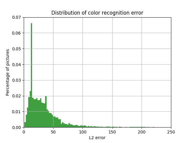
The distribution of the share of cars with the value of L2 error in the LAB space between the color at the output of the neural network, and the color of the car bounding box of the magnitude of this error
Examples
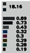
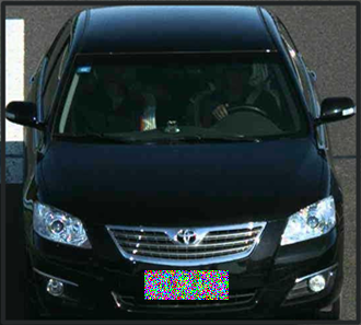
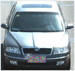
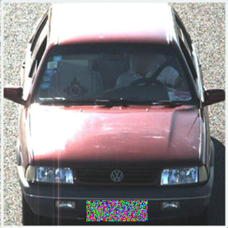
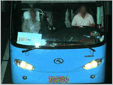
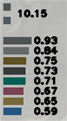
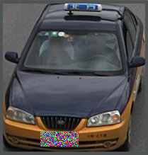
The following are examples of color recognition cars. The first - the black car (a typical case) is recognized as black, and the distance in the LAB space between the true color and a certain (18.16) is less than the minimum distance between the classes (28). In the second picture, the network was able not only to determine that the car is lit (there is a high probability that corresponds to one of the classes of white flowers), but also its real color (silver). However, the machine from the next figure, also illuminated, was not detected by the network as red. The color of the car shown in the figure below could not be determined at all by the network, which follows from the fact that the probabilities for all colors are too small.
In many ways, the task was due to the need to recognize multi-color cars. The last figure shows a two-tone black and yellow car. The black network is most likely recognized by the network, which is apparently due to the prevalence of machines of this and similar colors in the training dataset, and the yellow color, which is close to the true one, entered the top 3.
 |  |
|---|
 |  |
|---|
 |  |
|---|
 |  |
|---|
 |  |
|---|
ROC curve: visualization and problems
So, at the output, we got a fairly high result on the metric. The following figure shows the ROC curves both for solving a problem with 8 classes, and for a problem with 810 classes, as well as solutions without using neural networks. It can be seen that the result is slightly different than the one that was written out earlier. The previous results were obtained using TensorFlow, the graphs below were obtained using the scikit-learn package.
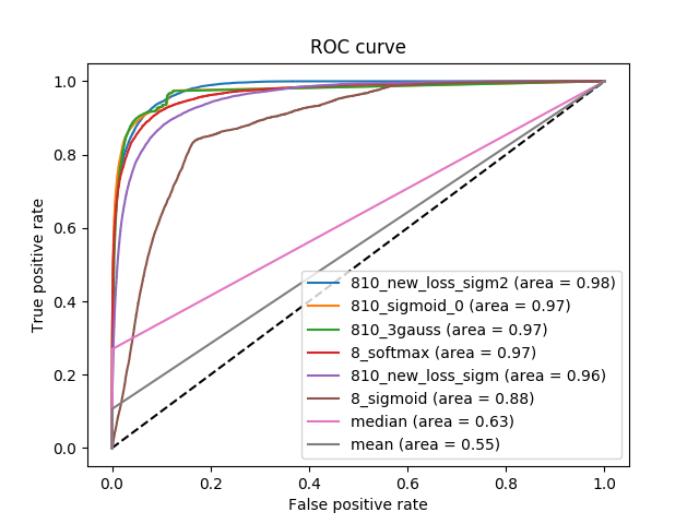 |  |
|---|
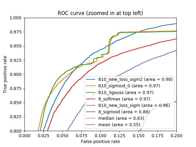
You can take any fixed numbers as threshold values (for example, Tensorflow when setting the corresponding parameter to 50 takes the same thresholds from 0 to 1 at regular intervals), you can - the values at the network output, or limit them from below to not consider values of the order of 10 -4 , for example. The result of the last approach is shown in the following figure.
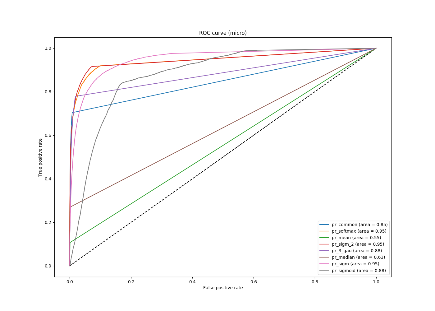
ROC curve for several solutions to a problem with a threshold of 10 -4.
It can be seen that all the curves that correspond to solving a problem using neural networks are characteristic better (are above) to solve the problem without them, but between the first you cannot choose one uniquely best curve. Depending on what threshold the user chooses, different curves will respond to different optimal solutions of the problem. Therefore, on the one hand, we have found such an approach, which allows us to determine the color of the car quite accurately and shows a high metric, on the other hand, we have shown that the limit has not yet been reached and the area metric under the ROC curve has its drawbacks.
Ready to answer questions and listen to comments in the comments.