The logic of thinking. Part 8. Isolation of factors in wave networks

In previous partswe described a model of a neural network, which we called a wave network. Our model is significantly different from traditional wave models. Usually, it is assumed that each neuron has its own oscillations. The joint work of such neurons prone to systematic pulsation in classical models leads to a certain general synchronization and the appearance of global rhythms. We put a completely different meaning in the wave activity of the cortex. We showed that neurons are able to capture information not only due to changes in the sensitivity of their synapses, but also due to changes in membrane receptors located outside the synapses. As a result, the neuron gains the ability to respond to a large set of specific patterns of activity of the surrounding neurons. We showed that the triggering of several neurons that form a specific pattern, necessarily triggers a wave propagating through the cortex. Such a wave is not just a perturbation transmitted from a neuron to a neuron, but a signal that creates as it moves a certain pattern of neuron activity, unique to each pattern that emits it. This means that in any place of the cortex, according to the pattern that the wave brought with it, it is possible to determine which patterns on the cortex came into activity. We have shown that through small bundles of fibers, wave signals can be projected onto other zones of the cortex. Now we will talk about how synaptic training of neurons in our wave networks can occur. unique to each pattern that emits it. This means that in any place of the cortex, according to the pattern that the wave brought with it, it is possible to determine which patterns on the cortex came into activity. We have shown that through small bundles of fibers, wave signals can be projected onto other zones of the cortex. Now we will talk about how synaptic training of neurons in our wave networks can occur. unique to each pattern that emits it. This means that in any place of the cortex, according to the pattern that the wave brought with it, it is possible to determine which patterns on the cortex came into activity. We have shown that through small bundles of fibers, wave signals can be projected onto other zones of the cortex. Now we will talk about how synaptic training of neurons in our wave networks can occur.

Isolation of wave factors

Take an arbitrary neuron of the cortex (Figure below). He has a receptive field within which he has a dense network of synaptic connections. These compounds encompass both surrounding neurons and axons entering the cortex that carry signals from other parts of the brain. Thanks to this, a neuron is able to monitor the activity of a small surrounding area. If the topographic projection falls on the cortical zone to which it belongs, then the neuron receives signals from those axons that fall into its receptive field. If there are active patterns of evoked activity on the cortex, then the neuron sees fragments of identification waves from them when they pass by it. Similarly with waves that arise from wave tunnels that carry the wave pattern from one area of ​​the brain to another.


Sources of information to highlight the factor. 1 - cortical neuron, 2 - receptive field, 3 - topographic projection, 4 - evoked activity pattern, 5 - wave tunnel

The main principle is observed in the activity visible by a neuron in its receptive field, regardless of its origin - each unique phenomenon causes its own unique inherent only to this phenomenon pattern. The phenomenon repeats - the pattern of activity visible to the neuron is repeated.

If what is happening contains several phenomena, then several patterns are superimposed on each other. When superimposed, the patterns of activity may not coincide in time, that is, the wave fronts can miss. To take this into account, we choose an indicative time interval equal to the period of one wave cycle. For each synaptic input of a neuron, we accumulate activity over this period of time. That is, we just sum up how many spikes came to this or that input. As a result, we obtain an input vector describing the picture of synaptic activity integrated over the cycle. Having such an input vector, we can use for the neuron all the previously described teaching methods. For example, we can turn a neuron into a Hebb filter and make it select the main component contained in the input data stream. In its essence, this will be the identification of those inputs on which most often incoming signals appeared together. As applied to identification waves, this means that the neuron will determine which waves have a pattern to appear together from time to time, and will set its weight to recognize this combination. That is, by highlighting such a factor, the neuron will begin to exhibit evoked activity when it recognizes the familiar combination of identifiers.

Thus, a neuron will acquire the properties of a neuron detector tuned to a specific phenomenon detected by its features. At the same time, the neuron will not only act as a presence sensor (there is a phenomenon - there is no phenomenon), it will signal the level of its activity about the severity of the factor for which it was trained. Interestingly, the nature of synaptic signals is not fundamental. With equal success, a neuron can tune in to the processing of wave patterns, patterns of topographic projection, or their joint activity.

It should be noted that the Hebb training, which distinguishes the first main component, is presented purely illustrative to show that the local receptive field of any cortical neuron contains all the necessary information for training it as a universal detector. Real algorithms for the collective training of neurons, which distinguish many diverse factors, are organized somewhat more complicated.

Stability - ductility

Hebb education is very clear. It is convenient to use to illustrate the essence of iterative learning. If we talk only about activating connections, then as the neuron learns, its weights are tuned to a specific image. For a linear adder, activity is determined:



The coincidence of the signal with the image that stands out on the synaptic balance causes a strong response of the neuron, the mismatch is weak. When teaching according to Hebb, we strengthen the weights of those synapses to which the signal arrives at the moments when the neuron itself is active, and weaken those weights at which there is no signal at that time.

To avoid the endless growth of weights, a standardizing procedure is introduced that keeps their sum within certain limits. Such logic leads, for example, to the Oia rule:



The most unpleasant thing in standard Hebb training is the need to introduce a learning rate coefficient, which must be reduced as the neuron learns. The fact is that if you do not do this, then the neuron, having learned to some kind of image, then, if the nature of the supplied signals changes, it will be retrained to highlight a new factor characteristic of the changed data stream. A decrease in the learning speed, firstly, of course, slows down the learning process, and secondly, it requires not obvious methods of controlling this decrease. Inaccurate handling of the speed of learning can lead to the "stiffness" of the entire network and immunity to new data.

All this is known as the stability-plasticity dilemma. The desire to respond to a new experience threatens to change the weights of previously trained neurons, while stabilization leads to the fact that the new experience ceases to affect the network and is simply ignored. You have to choose either stability or ductility. To understand what mechanisms can help in solving this problem, let us return to biological neurons. Let us examine in more detail the mechanisms of synaptic plasticity, that is, with what the synaptic training of real neurons occurs at.

The essence of the phenomenon of synaptic plasticity is that the efficiency of synaptic transmission is not constant and can vary depending on the pattern of current activity. Moreover, the duration of these changes can vary greatly and be caused by different mechanisms. There are several forms of plasticity (figure below).


The dynamics of synaptic sensitivity. (A) - facilitation, (B) - amplification and depression, (C) - post-tetanic potency (D) - long-term potency and long-term depression (Nicholls J., Martin R., Wallas B., Fuchs P., 2003)

A short volley of spikes can cause relief (facilitation) of the release of the mediator from the corresponding presynaptic terminal. Facilitation appears instantly, persists during a volley and is noticeably noticeable for about 100 milliseconds after the end of stimulation. The same short exposure can lead to suppression (depression) of the release of the mediator, lasting several seconds. Facilitation can go into the second phase (amplification), with a duration similar to the duration of depression.

A continuous high-frequency series of pulses is usually called a tetanus. The name is due to the fact that a similar series precedes tetanic muscle contraction. The intake of the tetanus at the synapse can cause a post-tetanic potency of mediator secretion, observed within a few minutes.

Repeated activity can cause long-term changes in synapses. One reason for these changes is an increase in the concentration of calcium in the postsynaptic cell. A strong increase in concentration triggers cascades of secondary messengers, which leads to the formation of additional receptors in the postsynaptic membrane and a general increase in receptor sensitivity. A weaker increase in concentration gives the opposite effect - the number of receptors decreases, their sensitivity decreases. The first condition is called long-term potency, the second - long-term depression. The duration of such changes is from several hours to several days (Nicholls J., Martin R., Wallas B., Fuchs P., 2003).

How the sensitivity of an individual synapse changes in response to external impulses, whether amplification will occur or depression will occur is determined by many processes. It can be assumed that this mainly depends on how the general picture of the neuron's excitation develops and what stage of training it is at.

The described behavior of synaptic sensitivity further suggests that the neuron is capable of the following operations:

• quickly tune in to a specific image - facilitation;
• reset this setting after an interval of the order of 100 milliseconds or transfer it to a longer hold - amplification and depression;
• reset the state of amplification and depression or translate them into long-term potency or long-term depression.

This phasing of learning is well correlated with the concept known as the “theory of adaptive resonance”. This theory was proposed by Stefan Grossberg (Grossberg, 1987), as a way to solve the stability-plasticity dilemma. The essence of this theory is that the incoming information is divided into classes. Each class has its own prototype - the image that most closely matches this class. For new information, it is determined whether it belongs to one of the existing classes, or whether it is unique, unlike anything previous. If the information is not unique, then it is used to clarify the prototype of the class. If this is something fundamentally new, a new class is created, the prototype of which is this image. This approach allows, on the one hand, to create new detectors, and on the other hand, not to destroy already created ones.



ART adaptive resonance network The

practical implementation of this theory is the ART network. At first, the ART network does not know anything. The first image submitted to her creates a new class. The image itself is copied as a class prototype. The following images are compared with existing classes. If the image is close to the already created class, that is, it causes resonance, then corrective training of the class image takes place. If the image is unique and does not resemble any of the prototypes, a new class is created, and the new image becomes its prototype.
If we assume that the formation of detector neurons in the cortex occurs in a similar way, then the following interpretation can be given to the phases of synaptic plasticity:

• a neuron that has not yet received specialization as a detector, but has come into activity due to wave activation, quickly changes the weight of its synapses, adjusting to the picture of the activity of its receptive field. These changes are in the nature of facilitation and continue on the order of one cycle of wave activity;
  
• if it turned out that in the immediate environment there are already enough neuron detectors tuned to such a stimulus, then the neuron is reset to its original state, otherwise its synapses go to the stage of a longer image retention;
  
• If during the amplification stage certain conditions are met, then the neuron synapses pass into the stage of long-term storage of the image. A neuron becomes a detector of the corresponding stimulus.
  

And now let's try to systematize a little about the training procedures that are relevant for artificial neural networks. Let's start with the learning objectives. We will assume that as a result of training we would like to receive neurons-detectors that satisfy two basic requirements:

• so that with their help it would be possible to fully and adequately describe everything that happens;
• for such a description to single out the basic laws inherent in current events.

The first allows, by remembering, to accumulate information without missing out on details that may subsequently turn out to be important patterns. The second provides the visibility of those factors in the description on which decision-making may depend.

The approach based on optimal data compression is well known. So, for example, using factor analysis, we can get the main components, which account for the bulk of the variability. Leaving the values ​​of the first few components and discarding the rest, we can significantly reduce the length of the description. In addition, the values ​​of the factors will tell us about the severity in the described event of the phenomena to which these factors correspond. But this compression also has a downside. For real events, the first major factors in the aggregate usually explain only a small percentage of the total variance. Each of their insignificant factors, although inferior many times in magnitude to the first factors, but it is the sum of these insignificant factors that is responsible for the basic information.

For example, if you take several thousand films and get their ratings put down by hundreds of thousands of users, then with such data you can conduct a factor analysis. The first four to five factors will be most significant. They will correspond to the main genre areas of cinema: action, comedy, melodrama, detective, science fiction. For Russian users, there will also be a strong factor that describes our old Soviet cinema. Highlighted factors have a simple interpretation. If you describe a film in the space of these factors, then this description will consist of coefficients saying how much this or that factor is expressed in this film. Each user has certain genre preferences that affect his rating. Factor analysis allows you to isolate the main directions of this influence and turn them into factors. But it turns out that the first significant factors account for only about 25% of the variance of estimates. All the rest is due to thousands of other small factors. That is, if we try to compress the description of the film to its portrait in the main factors, we will lose the bulk of the information.

In addition, one cannot talk about the unimportance of factors with little explanatory power. So, if you take several films of one director, then their estimates are likely to be closely correlated with each other. The relevant factor will explain a significant percentage of the variance in the ratings of these films, but only these. This means that since this factor does not appear in other films, its explanatory percentage in the entire amount of data will be negligible. But it is for these films that it will be much more important than the first main components. And so for almost all small factors.

The reasoning given for factor analysis can be shifted to other methods of coding information. David Field, in a 1994 article, “What is the Purpose of Sensory Coding?” (Field, 1994) addressed similar questions regarding the mechanisms inherent in the brain. He concluded that the brain does not compress data and does not strive for a compact form of data. The brain is more comfortable with their discharged representation, when having many different attributes to describe it, it simultaneously uses only a small part of them (Figure below).


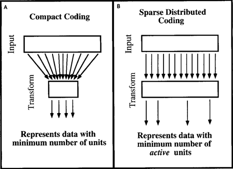
Compact coding (A) and economical distributed coding (B) (Field, 1994)

Both factor analysis and many other methods of description are repelled by the search for certain laws and the identification of the corresponding factors or signs of classes. But often there are data sets where this approach is practically not applicable. For example, if we take the clockwise position, it turns out that she has no preferred directions. It moves evenly on the dial, counting hour by hour. In order to convey the position of the arrow, we do not need to highlight any factors, and they will not stand out, but simply divide the dial into the corresponding sectors and use this partition. A large part of the brain deals with data that does not imply division, taking into account the distribution density of events, but simply requires the introduction of some kind of interval description. Actually

Isolation of the main components or fixation of adaptive resonance prototypes is far from all methods that allow neural networks to train neuron detectors convenient for the formation of description systems. Actually, any method that allows either to obtain a healthy division into groups, or to highlight some regularity, can be used by a neural network that reproduces the cerebral cortex. It seems that the real crust exploits many different methods, not limited to those that we cited as an example.

While we were talking about training individual neurons. But the main information element in our networks is the pattern of neurons, only it is able to start its own wave. A single neuron in a field is not a warrior. In the next part, we will describe how neural patterns corresponding to certain phenomena can arise and work.

Used literature

Continuation

Previous parts:
Part 1. Neuron
Part 2. Factors
Part 3. Perceptron, convolutional networks
Part 4. Background activity
Part 5. Brain waves
Part 6. Projection system
Part 7. Human-computer interface