The book "Deep learning on R"

Deep learning - Deep learning is a set of machine learning algorithms that model high-level abstractions in data using architectures made up of many non-linear transformations. Agree, this phrase sounds ominously. But everything is not so bad if Francois Chollet, who created Keras, the most powerful library for working with neural networks, tells us about deep learning. Get to know deep learning from practical examples from a wide variety of fields. The book is divided into two parts, in the first are the theoretical foundations, the second is devoted to solving specific problems. This will allow you to not only understand the basics of DL, but also learn how to use the new features in practice. This book is written for people with R programming experience who want to quickly learn deep learning in practice,

About this book

The book “Deep Learning in R” is addressed to statisticians, analysts, engineers and students with R programming skills, but not having significant knowledge in the field of machine and deep learning. This book is a revised version of the previous book, Deep Learning in Python , containing examples that use the R interface for Keras. The purpose of this book is to provide the R community with a guide containing everything you need, from basic theory to advanced practical applications. You will see more than 30 examples of program code with detailed comments, practical recommendations and simple generalized explanations of everything you need to know to use in-depth training in solving specific problems.

The examples use the Keras deep learning framework and the TensorFlow library as an internal mechanism. Keras is one of the most popular and rapidly developing deep learning frameworks. It is often recommended as the most successful tool for beginners to learn deep learning. After reading this book, you will understand what deep learning is, for what tasks this technology can be involved and what limitations it has. You will become familiar with the standard process of interpreting and solving machine learning problems and learn how to deal with typical problems. You will learn how to use Keras to solve practical problems from pattern recognition to natural language processing: image classification, prediction of time sequences, analysis of emotions and generation of images and text, and much more.

Excerpt 5.4.1. Visualization of intermediate activations

The visualization of intermediate activations consists in displaying the feature maps that are output by different convolutional and unifying levels in the network in response to certain input data (level output, the result of the activation function, often called its activation). This technique allows you to see how the input data is decomposed into various filters received by the network in the learning process. Typically, feature maps are used for visualization with three dimensions: width, height, and depth (color channels). Channels encode relatively independent features, therefore, in order to visualize these feature maps, it is preferable to build two-dimensional images for each channel separately. Let's start by loading the model saved in section 5.2:

> library(keras)> model <- load_model_hdf5("cats_and_dogs_small_2.h5")> model________________________________________________________________Layer (type)              Output Shape                                 Param #
==============================================================
conv2d_5 (Conv2D)   (None, 148, 148, 32)  896
________________________________________________________________
maxpooling2d_5        (MaxPooling2D) (None, 74, 74, 32)   0
________________________________________________________________
conv2d_6 (Conv2D)   (None, 72, 72, 64)                           18496
________________________________________________________________
maxpooling2d_6        (MaxPooling2D) (None, 36, 36, 64)   0
________________________________________________________________
conv2d_7 (Conv2D)   (None, 34, 34, 128)                         73856
________________________________________________________________
maxpooling2d_7        (MaxPooling2D) (None, 17, 17, 128)  0
________________________________________________________________
conv2d_8 (Conv2D)   (None, 15, 15, 128)                          147584
________________________________________________________________
maxpooling2d_8        (MaxPooling2D) (None, 7, 7, 128)      0
________________________________________________________________
flatten_2 (Flatten)      (None, 6272)                                   0
________________________________________________________________
dropout_1 (Dropout)  (None, 6272)                                    0
________________________________________________________________
dense_3 (Dense)        (None, 512)                                     3211776
________________________________________________________________
dense_4 (Dense)        (None, 1)                                         513
================================================================
Total params: 3,453,121
Trainable params: 3,453,121
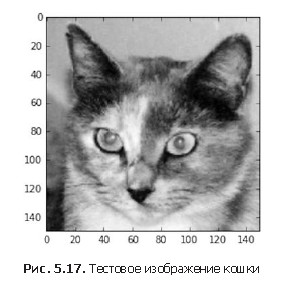
Non-trainable params: 0

Next, select the input image of the cat, which is not part of the training set.


Listing 5.25. Display test image

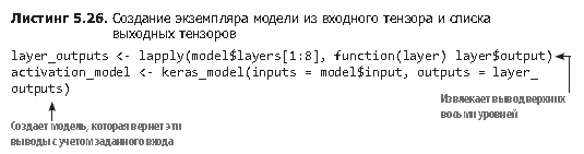
plot(as.raster(img_tensor[1,,,]))

To extract feature maps to be visualized, create a Keras model that accepts image packets and displays the activation of all convolutional and unifying levels. To do this, use the keras_model function from the Keras framework, which takes two arguments: an input tensor (or a list of input tensors) and an output tensor (or a list of output tensors). The result is a Keras model object, similar to the models, returned by the keras_sequential_model () function that you are already familiar with; This model maps the specified input to the specified output. A feature of
this type of model is the ability to create models with multiple outputs (unlike keras_sequential_model ()). The keras_model function is discussed in more detail in section 7.1.



If you transfer an image to this model, it will return the activation values ​​of the layers in the original model. This is the first example of a model with several outputs in this book: until now, all the models presented above had exactly one input and one output. In general, a model can have any number of inputs and outputs. In particular, this model has one input and eight outputs: one for each level activation.


Take for example the activation of the first convolutional layer for the input image of the cat:

> first_layer_activation <- activations[[1]]
> dim(first_layer_activation)
[1] 114814832

This is a feature map of 148 × 148 with 32 channels. Let's try to display some of them. First, we define a function to visualize the channel.

Listing 5.28. Channel visualization function

plot_channel <- function(channel){
rotate <- function(x)t(apply(x, 2, rev))image(rotate(channel), axes = FALSE, asp = 1,
col = terrain.colors(12))
}

Now let's display the second channel of activation of the first level of the original model (Fig. 5.18). It looks like this channel is a contour detector.
Listing 5.29. Visualization of the second channel

plot_channel(first_layer_activation[1,,,2])

Now look at the seventh channel (Fig. 5.19), but keep in mind that your channels may differ, because the training of specific filters is not a deterministic operation. This channel is slightly different and it looks like it gives off cat's eye iris.
Listing 5.30. Channel 7 Visualization

plot_channel(first_layer_activation[1,,,7])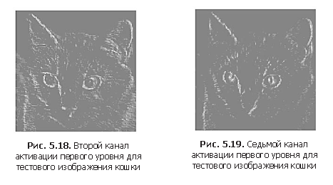

Now we will build a full visualization of all activations in the network (Listing 5.31). To do this, we extract and display each channel in all eight activation cards, placing the results in one larger tensor with images (Fig. 5.20–5.23).

Listing 5.31. Visualization of all channels for all intermediate activations

image_size <- 58
images_per_row <- 16for (i in1:8) {
   layer_activation <- activations[[i]]
   layer_name <- model$layers[[i]]$name
   n_features <- dim(layer_activation)[[4]]
   n_cols <- n_features %/% images_per_row
   png(paste0("cat_activations_", i, "_", layer_name, ".png"),
          width = image_size * images_per_row,
          height = image_size * n_cols)
   op <- par(mfrow = c(n_cols, images_per_row), mai = rep_len(0.02, 4))
   for (col in0:(n_cols-1)) {
      for (row in0:(images_per_row-1)) {
         channel_image <- layer_activation[1,,,(col*images_per_row) + row + 1]
         plot_channel(channel_image)
      }
   }
   par(op)
   dev.off()
}

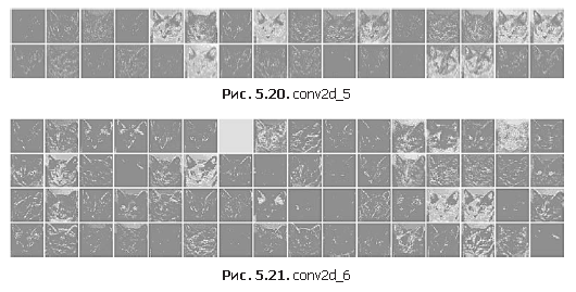
Here are a few comments on the results.

• The first layer acts as a collection of different contour detectors. At this stage, the activation saves almost all the information available in the original image.
• As you climb up the layers of activation, they become more and more abstract, and their visual interpretation becomes more and more complex. They begin to encode higher-level concepts, such as cat's ear or cat's eye. High-level views carry less and less information about the original image and more about the image class.
• The sparsity of activations increases with the depth of the layer: in the first layer, all filters are activated by the original image, but in subsequent layers, more and more empty filters remain. This means that the pattern corresponding to the filter is not found in the original image.

We have just considered an important universal characteristic of representations created by deep neural networks: the features extracted by layers become more and more abstract with the depth of the layer. Activations on the upper layers contain less and less information about a particular input image, and more and more about the target (in this case, about the image class - a cat or a dog). A deep neural network actually acts as an information cleaning pipeline that receives raw data that is not cleaned (in this case, RGB images) and subjected to multiple transformations, filtering unnecessary information (for example, the specific appearance of an image) and leaving Images).

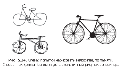
People and animals perceive the world around in the same way: after observing the scene for a few seconds, a person remembers which abstract objects are present in it (bicycle, tree), but does not remember all the details of the appearance of these objects. In fact, when you try to draw a bicycle from memory, you most likely will not be able to get a more or less correct image, even though you could see bicycles a thousand times (see examples in Figure 5.24). Try to do it right now and you will be convinced of the truth of what has been said. Your brain has learned to completely abstract the visible image received at the input, and transform it into high-level visual concepts, while filtering unimportant visual details, making it difficult to remember them.



»More information about the book is available on the publisher's website
» Table of contents
» Excerpt

For Habrozhiteley 20% discount on the coupon - Deep Learning with R