Data Modeling in Cassandra 2.0 in CQL3
- Tutorial
This article is intended for people trying to create their first “table” in the Cassandra database.
For posting several releases of Cassandra, the developers took the right vector aimed at the ease of use of this database. Given its advantages, such as speed and fault tolerance, it was difficult to administer and write for it. Now the number of dances with a tambourine that needs to be done before starting and starting to develop has been minimized - a few commands in bash or one .msi in Windows.
Moreover, the recently updated CQL (query language) made life easier for developers, displacing the binary and rather complex language Thrift.
Personally, I was faced with the problem of the absence of Russian-language manuals on Kassandra. In my opinion, the most difficult topic I would like to raise in this article. How to design a database then?
Kassandra was created as a distributed database with an emphasis on maximum write and read speeds. You need to model the “tables” depending on the
In SQL, we are used to throwing tables, relationships between them, and then
We have employees of some company. Let's create a table (which are actually called the Column Family, but for ease of transition from SQL to CQL use the word table) in CQL and fill it with data:
Tables in C * must have a PRIMARY KEY. It is used to search for the node in which the search string is stored.
Read the data:
This picture is the hand-decorated cqlsh output.

It looks like a regular table from a relational database. C * will create two lines.

Attention! These are two internal row structures , not tables. If a little cunning, then we can say that each row is like a small table. Further clear.
Complicate. Add the company name.
Read the data:

Attention to the PRIMARY KEY. The first parameter is
This is how the internal structure now looks .
As you can see with us:
Even harder. The capital letter is the name of the column. Lowercase - data.
Read the data:
Now our distribution key is composite
internal structure has become more complicated. Such data as
This is the fastest way to record and store an infinite amount of data in a distributed database. C * was just designed with an emphasis on write / read speed. Here, for example, compares MongoDB, HBase, and C * speeds .
We have some events that occur 1000 times per second. For example, indicators are taken from noise level sensors. 10 sensors. Each of them sends data 100 times per second. We have 3 tasks:
We need to install several nodes, make each autonomous. It can even take one of them into the cloud.
We will store the data of one day in one line.
Since the distribution key is a unique combination of day + sensor, the data for one day will be stored for each sensor in a separate line. Thanks to reverse sorting inside the string, we get the most important (last) data for us “at the fingertips”.
Since the search for the distribution key (day) is a very fast operation in C *, the third point can be considered completed.
Of course, we can do a day / day search, and inside the day already compare the timestamp. But there can be many days.
After all, we have only 10 sensors. Is it possible to use this? It is possible, if you imagine that one sensor is one line. In this case, C * caches in memory the location of all ten lines on the disk.
Create a second table, where we will store the same data, but excluding days.
And when we insert the data, we will limit the lifetime of each cell so as not to get used to 2 billion columns. With us, each sensor gives no more than 100 readings per second. Hence:
We must make sure that after 248 days the oldest data is quietly and quietly deleted.
In the application code, it will be necessary to set the condition that if the requested data goes beyond the last 248 days, then we use the table
“What nonsense! Why a second table? ”You will think. I repeat: in the C * database, storing the same value several times is the norm, the correct model. The winnings are as follows:
I recommend viewing it in this order.
UPD: Correction of terminology. Replaced the words "master key" with "distribution key" in the right places. Added in some places the concept of "cluster key".
For posting several releases of Cassandra, the developers took the right vector aimed at the ease of use of this database. Given its advantages, such as speed and fault tolerance, it was difficult to administer and write for it. Now the number of dances with a tambourine that needs to be done before starting and starting to develop has been minimized - a few commands in bash or one .msi in Windows.
Moreover, the recently updated CQL (query language) made life easier for developers, displacing the binary and rather complex language Thrift.
Personally, I was faced with the problem of the absence of Russian-language manuals on Kassandra. In my opinion, the most difficult topic I would like to raise in this article. How to design a database then?
Disclaimer
- The article is NOT intended for people who first see the word Cassandra.
- The article does NOT serve as an advertising material for a particular technology.
- The article does NOT seek to prove anything to anyone.
- If the write / read speed is not so important, and if “100% uptime” is not really needed, and if you have only a few million records, then probably this article, and the whole Cassandra as a whole, is not what you necessary.
Educational program
- Cassandra (hereinafter C * ) is a distributed NoSQL database, therefore all decisions “why so, and not like this” are always made with an eye to clustering.
- CQL is an SQL-like language. Abbreviation for C assandra Q uery L anguage.
- Node is a C * instance, or java process in terms of operating systems. You can run multiple nodes on the same machine, for example.
- The basic storage unit is a string . The whole string is stored on nodes, i.e. There are no situations when half a line is on one node, half a line is on another. A row can dynamically expand to 2 billion columns. It is important.
- cqlsh - command line for CQL. All the examples below are executed in it. It is part of the C * distribution.
Basic Data Modeling Rule in C *
Kassandra was created as a distributed database with an emphasis on maximum write and read speeds. You need to model the “tables” depending on the
SELECTrequests of your application . In SQL, we are used to throwing tables, relationships between them, and then
SELECT ... JOIN ...what we want and how we want. It is JOINs that are the main problem with performance in RDBMS. They are not in CQL.The first example.
We have employees of some company. Let's create a table (which are actually called the Column Family, but for ease of transition from SQL to CQL use the word table) in CQL and fill it with data:
CREATE TABLE employees (
    name text, -- уникальное имя
    age int, -- какие-то данные про человека
    role text, -- ещё какие-то данные
    PRIMARY KEY (name)); -- обязательная часть любой таблицы
INSERT INTO employees (name, age, role) VALUES ('john', 37, 'dev');
INSERT INTO employees (name, age, role) VALUES ('eric', 38, 'ceo');
Tables in C * must have a PRIMARY KEY. It is used to search for the node in which the search string is stored.
Read the data:
SELECT * FROM employees;
This picture is the hand-decorated cqlsh output.
It looks like a regular table from a relational database. C * will create two lines.
Attention! These are two internal row structures , not tables. If a little cunning, then we can say that each row is like a small table. Further clear.
Second example.
Complicate. Add the company name.
CREATE TABLE employees (
  company text,
  name text,
  age int,
  role text,
  PRIMARY KEY (company,name) -- две части главного ключа: распределительный ключ company и кластерный ключ name
);
INSERT INTO employees (company, name, age, role) VALUES ('OSC', 'eric', 38, 'ceo');
INSERT INTO employees (company, name, age, role) VALUES ('OSC', 'john', 37, 'dev');
INSERT INTO employees (company, name, age, role) VALUES ('RKG', 'anya', 29, 'lead');
INSERT INTO employees (company, name, age, role) VALUES ('RKG', 'ben', 27, 'dev');
INSERT INTO employees (company, name, age, role) VALUES ('RKG', 'chan', 35, 'ops');
Read the data:
SELECT * FROM employees;
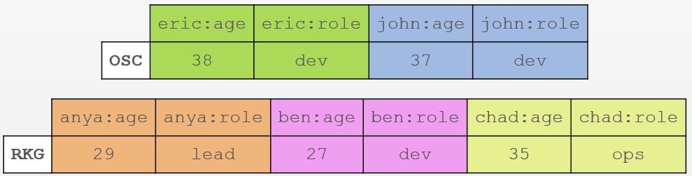
Attention to the PRIMARY KEY. The first parameter is
companythe distribution key; it will be used to search for the node from then on. The second key name- a cluster key (clustering key). He turns into a column. Those. we turn the data into the column name. It was 'eric' with the usual four bytes, and became part of the column name. This is how the internal structure now looks .
As you can see with us:
- Two companies -
OSCandRKG. Only two lines were created here. - Green
ericstores its age and role in two cells. Similarly, everyone else. - It turns out that with such a structure, we can store 1 billion employees in each company (line). Remember that the limit on the number of columns is 2 billion?
- It may seem that we are once again storing the same data. This is true, but in C * such a design is the correct modeling pattern.
- Expanding strings is the main feature when modeling in C *.
The third example.
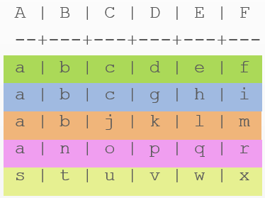
Even harder. The capital letter is the name of the column. Lowercase - data.
CREATE TABLE example (
  A text,
  B text,
  C text,
  D text,
  E text,
  F text,
  PRIMARY KEY ((A,B), C, D)); -- составной распределительный ключ (A,B) и кластерные ключи (C,D)
INSERT INTO example (A, B, C, D, E, F) VALUES ('a', 'b', 'c', 'd', 'e', 'f');
INSERT INTO example (A, B, C, D, E, F) VALUES ('a', 'b', 'c', 'g', 'h', 'i');
INSERT INTO example (A, B, C, D, E, F) VALUES ('a', 'b', 'j', 'k', 'l', 'm');
INSERT INTO example (A, B, C, D, E, F) VALUES ('a', 'n', 'o', 'p', 'q', 'r');
INSERT INTO example (A, B, C, D, E, F) VALUES ('s', 't', 'u', 'v', 'w', 'x');
Read the data:
SELECT * FROM example;
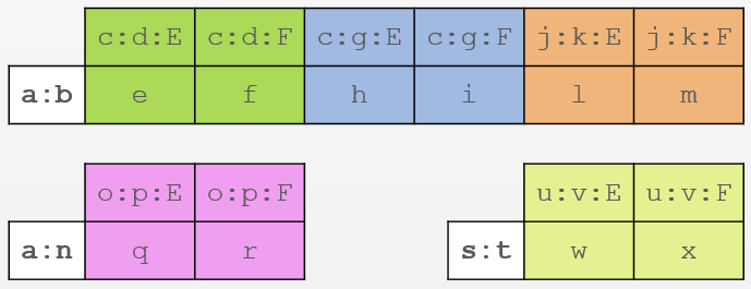
Now our distribution key is composite
(A,B). The cluster key is also composite - C, D. The internal structure has become more complicated. Such data as
c, d, g, k, o, p, u, vparticipating in the name of the columns along with E and F:- As you can see, now each unique combination of A and B is a key to the string.
- We have only three unique distribution keys -
a:b,a:nands:t. - Columns multiplied thanks to cluster keys. In the line
a:bwe have three unique combinations -c:d,c:g,j:k- are stored in columns E and F data itself -eandf,handi,landm. - Similarly two other lines.
Why is it so complicated?
This is the fastest way to record and store an infinite amount of data in a distributed database. C * was just designed with an emphasis on write / read speed. Here, for example, compares MongoDB, HBase, and C * speeds .
Real life example
We have some events that occur 1000 times per second. For example, indicators are taken from noise level sensors. 10 sensors. Each of them sends data 100 times per second. We have 3 tasks:
- Continue to write if the database server (node) stops its work.
- To manage to record 1000 new records in a second no matter what.
- Provide a graph of any sensor for any day in a couple of milliseconds.
- Provide a graph of any sensor for any period of time as quickly as possible.
The first and second points are easy.
We need to install several nodes, make each autonomous. It can even take one of them into the cloud.
The third point is the main trick.
We will store the data of one day in one line.
CREATE TABLE temperature_events_by_day (
  day text, -- Text of the following format: 'YYYY-MM-DD'
  sensor_id uuid,
  event_time timestamp,
  temperature double,
  PRIMARY KEY ((day,sensor_id), event_time) -- составной распред. ключ (day,sensor_id) и кластерный ключ (event_time)
)
WITH CLUSTERING ORDER BY event_time DESC; -- обратная сортировка записываемых данных
Since the distribution key is a unique combination of day + sensor, the data for one day will be stored for each sensor in a separate line. Thanks to reverse sorting inside the string, we get the most important (last) data for us “at the fingertips”.
Since the search for the distribution key (day) is a very fast operation in C *, the third point can be considered completed.
Fourth point
Of course, we can do a day / day search, and inside the day already compare the timestamp. But there can be many days.
After all, we have only 10 sensors. Is it possible to use this? It is possible, if you imagine that one sensor is one line. In this case, C * caches in memory the location of all ten lines on the disk.
Create a second table, where we will store the same data, but excluding days.
CREATE TABLE temperature_events (
  sensor_id uuid,
  event_time timestamp,
  temperature double,
  PRIMARY KEY (sensor_id, event_time) -- распределительный ключ (sensor_id) и кластерный ключ (event_time)
)
WITH CLUSTERING ORDER BY event_time DESC; -- обратная сортировка записываемых данных
And when we insert the data, we will limit the lifetime of each cell so as not to get used to 2 billion columns. With us, each sensor gives no more than 100 readings per second. Hence:
2**31 / (24 часа * 60 мин * 60 сек * 100 событий/сек) = 2147483648 / (24 * 60 * 60 * 100) = 248.55 днейWe must make sure that after 248 days the oldest data is quietly and quietly deleted.
INSERT INTO temperature_events (sensor_id, event_time, temperature)
VALUES ('12341234-1234-1234-123412', 2535726623061, 36.6)
TTL 21427200; -- 248 days in seconds
In the application code, it will be necessary to set the condition that if the requested data goes beyond the last 248 days, then we use the table
temperature_events_by_day, if not - temperature_events. Searching for the latter will be several milliseconds faster. “What nonsense! Why a second table? ”You will think. I repeat: in the C * database, storing the same value several times is the norm, the correct model. The winnings are as follows:
- Writing data to the second table is faster than the first. Cassandra will not have to look for the node (s) into which to add a new value. She will know in advance.
- Reading data is also very fast. For example, it is many times superior to a regular indexed, normalized SQL database.
Sources
I recommend viewing it in this order.
- Webinar - Understanding How CQL3 Maps to Cassandra's Internal Data Structure .
- Webinar - The Data Model is Dead, Long Live the Data Model
- Webinar - Become a Super Modeler
- Webinar - The World's Next Top Data Model
- Full CQL3 Documentation - Cassandra Query Language (CQL) v3
The next article in the series .
UPD: Correction of terminology. Replaced the words "master key" with "distribution key" in the right places. Added in some places the concept of "cluster key".