Sawing data with comfort

Good day time.
In actual practice, you often come across tasks that are far from complex ML algorithms, but are no less important and vital for business.
Let's talk about one of them.
The task is to distribute (cut, sprinkle - business jargon inexhaustible) the data of some target table with aggregates (aggregate values) on a table of more detailed granularity.
For example, the commercial department needs to split the annual plan agreed at the brand level - in detail before production, marketers break the annual marketing budget for the country's territories, the planning and economic department break the general economic costs by financial responsibility centers, etc. etc.
If you feel that tasks like this already loom in front of you on the horizon or already treat the victims of such tasks, then I ask for cat.
Consider a real-life example:
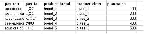
As a task, the sales plan is lowered as in the picture below (I deliberately made the example simplified, in reality, the cloth in Excel is 100–200 MGB).
Explanation of titles:
- pos_terr-territory (region) of the outlet
- pos_fo - the federal district of the outlet (for example, the CFA-Central Federal District)
- product_brend - product brand
- product_class - product class
- plan.sales is a sales plan for anything.
And they ask, for example, to break their mega-table (as part of our children's example, it is certainly more modest) - to the sales channel. To the question of what logic to break, I get the answer: “But take the statistics of actual sales for the 4th quarter of such a year, get the actual channel shares in% for each line of the plan and break these lines by these fractions”.
In fact, this is the most frequent answer in such tasks ...
So far everything seems simple enough.
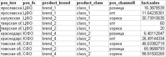
I get this fact (see the picture below):
- pos_channell - sales channel (target attribute for the plan)
- fact.sales - the actual sales of something.
Based on the received approach to “sawing” using the example of the first line of the plan, we divide it on the basis of the fact in some way:

However, if we compare the fact with the plan for the whole plate in order to understand whether all the lines of the plan will be adequately “sawn” in fractions we get the following picture: (green - all the attributes of the plan line coincided with the fact, the yellow cells did not match).
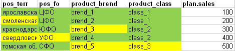
- In the 1st line of the plan, all the fields are completely found in the fact.
- Corresponding territory is not found in the 2nd line of the plan.
- In the 3rd line of the plan is missing in the fact of the brand.
- In the 4th line of the plan there is not enough in the fact of the territory and the federal district
- In the 5th line of the plan is missing in the fact of the brand and class.
As Panikovsky said: “Saw Shura, saw - they are golden ...”

I go to the business customer and check on the 2nd line, what approach does he see for such situations?
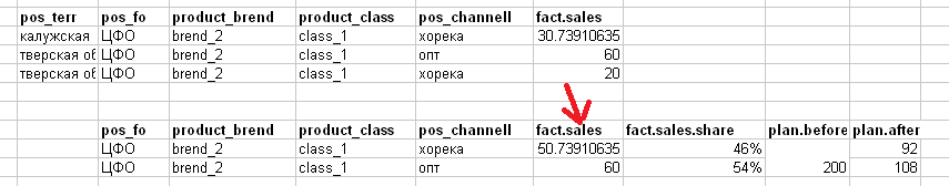
Get the response: "in cases where it is impossible to calculate the share of the channels for the brand № 2 in the Smolensk region (taking into account that the Smolensk region, we in the Central Federal District, Central Federal District) - break then this line of the channel structure within the entire CFD!"
That is, for {Smolensk region + brand_2} we aggregate the fact at the level of the Central Federal District and break the Smolensk region somehow like this:
Returning and digesting what I heard, I try to generalize to a more universal heuristic:
If there is no data at the current level of detail of the fact table, before calculating the shares for the target field (sales channel), we aggregate the fact table before the hierarchy attribute is higher.
That is, if there is no territory, then we aggregate the fact to the hierarchy level above - the shares for the same CFD as in the plan. If not for a brand, then according to the hierarchy above there is a class of a product - respectively, we recalculate the shares for the same class and so on.
Those. we combine the plan and the fact according to the coupling fields for which we count the shares in the fact and at each iteration of the remaining undisclosed plan we consistently reduce the composition of the coupling fields.
There is already a certain pattern of data distribution:
- We distribute the plan in fact based on the full coincidence of the corresponding fields
- We get a broken plan (we accumulate it into an intermediate result) and an unbroken plan (not all the lines coincided)
- We take an unbroken plan and break it down into a higher hierarchy level (i.e., discard the specific linkage field of these 2 tables and aggregate the fact without this field to calculate the shares)
- We get a broken plan (we add it to the intermediate result) and an unbroken plan (not all the lines coincided)
- And we repeat the same steps until there is an “uncut” plan.
In general, no one obliges us to consistently delete coupling fields only within the hierarchy. For example, we have already removed the brand and territory from the coupling fields, and the remaining plan was distributed according to: product_class (hierarchy is higher than brand) + Fed.krug (hierarchy is higher than territory). And still got some unallocated balance of the plan.
Then we can remove from the coupling fields either a product class or a federal district, since they are no longer invested in the hierarchy of each other.
Considering that tens of fields and lines in such tables — up to a million — to do such manipulations with your hands is not a pleasant task.
And if we take into account that tasks of this kind come to me regularly at the end of each year (approval of budgets of the next year on the board of directors), then we had to transfer this process to some flexible universal template.
And since most of the time I work with data through R, the implementation is accordingly the same on it.
To begin, we need to write a universal magic function that will accept the base table (basetab) with the data for the breakdown (in our example, the plan) and the table for calculating the shares (sharetab) on the basis of which we will “cut” the data (in our example, fact). But the function must also understand what to do with these objects, so the function will still accept the vector of the fields of the hitch (merge.vrs) - i.e. those fields that are equally named in both tables and allow us to join one table with another by these fields where it will turn out (i.e. right join). Also, the function must understand which column of the base table must be taken in the distribution (basetab.value) and on the basis of which field the shares are counted (sharetab.value). And the most important thing is what to take for the resulting field (sharetab.targetvars),
By the way, this variable sharetab.targetvars is not accidental in my plural - it can be not one field but a vector name field vector, for cases when you need to add more than one field from the table of shares from the table of shares (for example, it’s not possible to split the plan only by sales channel but also by the name of the products included in the brand).
Yes, and one more condition :) my function should be as concise and readable as possible, without any multi-storey on 2 screens (I really don't like big functions).
The popular dplyr package fit into the last condition as comfortably as possible, and given that its pipeline operators must understand the textual names of the fields that are lowered into the function - it was not without the Standart evaluation .
Here is this baby (not counting the internal comments):
fn_distr <- function(sharetab,  sharetab.value, sharetab.targetvars,  basetab, basetab.value, merge.vrs,level.txt=NA) {
  # sharetab - объект=таблица драйвер распределения
  # sharetab.value -  название поля с числами по которому будет пересчет в доли из таблицы-драйвер
  # sharetab.targetvars -  название целевого текстового поля из таблицы-драйвер по которому будет дробится базовая таблица на основе долей
  # basetab - объект=таблица с базовыми показателями к распределению
  # basetab.value - название поля с числами которые должны быть распределены
  # merge.vrs - название полей объединения 2-х таблиц
  # level.txt - примечание пользователя для тек.итерации чтобы можно было обосновать строку результата (если пользователь не указал то merge.vrs)
  require(dplyr)
  sharetab.value <- as.name(sharetab.value)
  basetab.value <- as.name(basetab.value)
  if(is.na(level.txt )){level.txt <- paste0(merge.vrs,collapse = ",")}
  result <- sharetab %>% group_by(.dots = c(merge.vrs, sharetab.targetvars)) %>% summarise(sharetab.sum = sum(!!sharetab.value)) %>% ungroup %>%
    group_by(.dots = merge.vrs) %>% mutate(sharetab.share = sharetab.sum / sum(sharetab.sum)) %>% ungroup %>%
    right_join(y = basetab, by = merge.vrs) %>% mutate(distributed.result = !!basetab.value * sharetab.share, level = level.txt) %>%
    select(-sharetab.sum,-sharetab.share)
  return(result)
}
At the output, the function should return the data.frame of joining two tables with those rows of the plan + fact where it was possible to split the current version of the coupling fields, and with the original rows of the plan (and empty fact) in the rows where the current iteration failed to split the plan.
That is, the result returned by the function after the first iteration (a breakdown of the first line of the plan for the Yaroslavl region) will look like this:
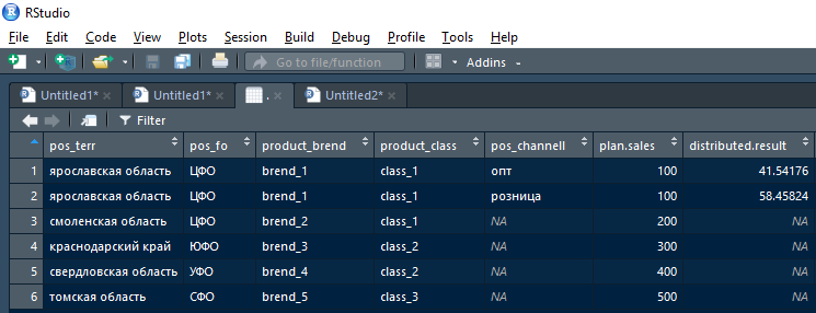
Then this result can be taken for non-empty distributed.result to the cumulative result and by empty (NA) distributed.result can be sent to the next one typical iteration but broken down by shares at a higher level of the hierarchy.
All the beauty and convenience is that the work goes on the same type of blocks and one universal function, all you need at each step (iteration) is to correct the vector merge.vrs and watch how the magic does all this tedious work for you:

Yes, I almost forgot a small nuance: if something goes wrong and at the very end we get a broken plan that will not be totally equal to the plan before the breakdown - it will be difficult to track at which iteration everything went wrong.
Therefore, each iteration is supplied with a checksum:
Сумма(План_изначальный)-Сумма(План_распределенный_в_накопленном результате)-Сумма(План_нераспределенный_после_тек.итерации)=0Now we will try to drive our example through the distribution template and see what we get at the output.
First, we will get the initial data:
library(dplyr)
plan <- data_frame(pos_terr = c("ярославская область", "смоленская область",
                                "краснодарский край", "свердловская область", "томская область"),
                   pos_fo = c("ЦФО", "ЦФО", "ЮФО", "УФО", "СФО"),
                   product_brend = c("brend_1", "brend_2", "brend_3", "brend_4", "brend_5"),
                   product_class = c("class_1",  "class_1", "class_2", "class_2", "class_3"),
                   plan.sales = c(100, 200, 300, 400, 500))
fact <- data_frame(pos_terr = c("ярославская область", "ярославская область",
                                "калужская область", "тверская область", "тверская область","краснодарский край", "краснодарский край",
                                "томская область", "томская область", "томская область"),
                   pos_fo = c("ЦФО", "ЦФО","ЦФО","ЦФО", "ЦФО", "ЮФО", "ЮФО", "СФО", "СФО", "СФО"),
                   product_brend = c("brend_1",  "brend_1", "brend_2", "brend_2","brend_2", "brend_4", "brend_4", "brend_1", "brend_2",  "brend_4"),
                   product_class = c("class_1", "class_1", "class_1","class_1","class_1",  "class_2", "class_2", "class_1", "class_1", "class_2"),
                   pos_channell = c("розница",  "опт", "хорека","опт", "хорека", "розница", "опт", "хорека", "розница", "хорека"),
                   fact.sales = c(16.38, 11.64, 30.73,60, 20, 6.40, 26.49, 46.63, 65.96,  98.81))
</soure>
Затем зарезервируем остаток нераспрделенного плана (пока что равен исходному) и пустой фрейм для результата.
<source>
plan.remain <- plan
result.total <- data_frame()
1. We distribute on terr, pho (fed.krug), brand, class
merge.fields <- c("pos_terr","pos_fo","product_brend", "product_class")
result.current <- fn_distr(sharetab = fact,sharetab.value = "fact.sales",sharetab.targetvars = "pos_channell",
                           basetab = plan.remain,basetab.value = "plan.sales",merge.vrs = merge.fields)
result.total <- result.current %>% filter(!is.na(distributed.result)) %>% select(-plan.sales) %>% bind_rows(result.total)
# ниже получаем остаток плана - нераспределенные записи для следующих итераций
plan.remain <- result.current %>% filter(is.na(distributed.result)) %>% select(colnames(plan))
# на каждой итерации проверяем что сумма оставшегося плана и накопительное распрделение = сумме исходного плана
cat("Расхождение :",sum(plan.remain$plan.sales)+sum(result.total$distributed.result)-sum(plan$plan.sales),"\n",
    "Осталось распределить:",nrow(plan.remain)," записей")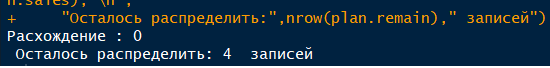
2. We distribute by pho, brand, class (ie, we refuse territory in fact).
The only difference from the first block is that the merge.fields were slightly shortened by removing pos_terr in it.
merge.fields <- c("pos_fo","product_brend", "product_class")
result.current <- fn_distr(sharetab = fact,sharetab.value = "fact.sales",sharetab.targetvars = "pos_channell",
                           basetab = plan.remain,basetab.value = "plan.sales",merge.vrs = merge.fields)
result.total <- result.current %>% filter(!is.na(distributed.result)) %>% select(-plan.sales) %>% bind_rows(result.total)
plan.remain <- result.current %>% filter(is.na(distributed.result)) %>% select(colnames(plan))
cat("Расхождение :",sum(plan.remain$plan.sales)+sum(result.total$distributed.result)-sum(plan$plan.sales),"\n",
    "Осталось распределить:",nrow(plan.remain)," записей")
3. Distributed by pho, class
merge.fields <- c("pos_fo", "product_class")
result.current <- fn_distr(sharetab = fact,sharetab.value = "fact.sales",sharetab.targetvars = "pos_channell",
                           basetab = plan.remain,basetab.value = "plan.sales",merge.vrs = merge.fields)
result.total <- result.current %>% filter(!is.na(distributed.result)) %>% select(-plan.sales) %>% bind_rows(result.total)
plan.remain <- result.current %>% filter(is.na(distributed.result)) %>% select(colnames(plan))
cat("Расхождение :",sum(plan.remain$plan.sales)+sum(result.total$distributed.result)-sum(plan$plan.sales),"\n",
    "Осталось распределить:",nrow(plan.remain)," записей")
4. Distributed by class
merge.fields <- c( "product_class")
result.current <- fn_distr(sharetab = fact,sharetab.value = "fact.sales",sharetab.targetvars = "pos_channell",
                           basetab = plan.remain,basetab.value = "plan.sales",merge.vrs = merge.fields)
result.total <- result.current %>% filter(!is.na(distributed.result)) %>% select(-plan.sales) %>% bind_rows(result.total)
plan.remain <- result.current %>% filter(is.na(distributed.result)) %>% select(colnames(plan))
cat("Расхождение :",sum(plan.remain$plan.sales)+sum(result.total$distributed.result)-sum(plan$plan.sales),"\n",
    "Осталось распределить:",nrow(plan.remain)," записей")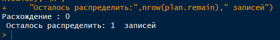
5. Distributed by FD
merge.fields <- c( "pos_fo")
result.current <- fn_distr(sharetab = fact,sharetab.value = "fact.sales",sharetab.targetvars = "pos_channell",
                           basetab = plan.remain,basetab.value = "plan.sales",merge.vrs = merge.fields)
result.total <- result.current %>% filter(!is.na(distributed.result)) %>% select(-plan.sales) %>% bind_rows(result.total)
plan.remain <- result.current %>% filter(is.na(distributed.result)) %>% select(colnames(plan))
cat("Расхождение :",sum(plan.remain$plan.sales)+sum(result.total$distributed.result)-sum(plan$plan.sales),"\n",
    "Осталось распределить:",nrow(plan.remain)," записей")
As we see, there is no “uncut” plan and the arithmetic of the distributed plan is equal to the original one.

And here is the result with sales channels (in the right column, the function outputs — according to which fields the hitch / aggregation went, so as to understand where this distribution comes from):

That's all. The article was not very small, but there is more explanatory text than the code itself.
I hope this flexible approach will save time and nerves not only for me :-)
Thank you for your attention.