What you wanted to know about optical flow, but were embarrassed to ask

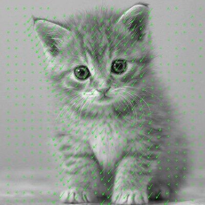
Optical flow (Optical flow) is a technology used in various areas of computer vision to determine shifts, segmentation, selection of objects, video compression. However, if we want to quickly implement it in our project by reading about it on Wikipedia or elsewhere, then we will most likely stumble on the fact that it works very poorly and fails when determining shifts already on the order of 1-2 pixels (at least it was with me). Then we turn to ready-made implementations, for example, in OpenCV. There it is implemented by various methods and it is completely incomprehensible why the abbreviation PyrLK is better or worse than the designation Farneback or something like that, and you have to deal with the meaning of the parameters, which in some implementations are very many. And, interestingly, these algorithms somehow work, unlike what we wrote ourselves. What is the secret?

What is optical flow?

Optical flow (OP) is an image of visible movement, which is a shift of each point between two images. In fact, it represents a velocity field (since a shift accurate to scale is equivalent to an instantaneous velocity). The essence of the OP is that for each point in the image there is such a shift (dx, dy) so that the point on the second image corresponds to the starting point. How to determine the correspondence of points is a separate issue. To do this, we need to take some function of the point, which does not change as a result of the displacement. It is usually believed that the point retains intensity (i.e., brightness or color for color images), but points that have the same gradient value, Hessian, its value or its determinant, Laplacian, and other characteristics can be considered identical. Obviously, maintaining the intensity fails if the illumination or angle of incidence of light changes. Nevertheless, if we are talking about a video stream, then, most likely, the lighting will not change much between the two frames, if only because a small period of time passes between them. Therefore, intensity is often used as a function that remains at a point.

According to such a description, the OP can be confused with the search and comparison of characteristic points. But these are different things, the essence of the optical stream is that it does not look for any special points, but tries to determine by the parameters of the images where an arbitrary point has moved.

There are two options for calculating the optical flux: dense (dense) and selective (sparse). Sparse stream calculates the shift of individual given points (for example, points selected by some feature detector), dense stream considers the shift of all points in the image. Naturally, the sample stream is calculated faster, but for some algorithms the difference is not so big, and for some tasks it is necessary to find the stream at all points of the image.

For degenerate cases, simpler methods for determining the shift can be applied. In particular, if all points of the image have the same shift (the entire image is shifted), then the phase correlation method can be applied: calculate the Fourier transform for both images, find the convolution of their phases and determine the shift from it (see en.wikipedia.org / wiki / Phase_correlation ). You can also use block matching: find a shift that minimizes the norm of the difference in the image in the window. In its pure form, such an algorithm will work for a long time and is unstable to bends and other distortions. English Wikipediaranks the above algorithms as different options for calculating the optical flow, but it seems to me not too correct, since these algorithms can be used for other purposes and do not completely solve this problem. We will call optical flow methods based on local characteristics of images (what is called differential methods in English Wikipedia).

Standard Approach (Lucas-Canada Method)

The mathematical description of the algorithm is given in sufficient detail in this article , but only theoretical aspects are affected.

Consider the mathematical model of the optical flow, assuming that the intensity of the point as a result of the displacement has not changed.

Let be the intensity at some point (x, y) in the first image (i.e., at time t). In the second image, this point shifted by (dx, dy), while the time dt passed, then - we expanded the intensity function according to Taylor to the first term (it will be mentioned later why only to the first), here are the partial derivatives with respect to coordinates and time , that is, in fact - a change in brightness at the point (x, y) between two frames.

We believe that the intensity has been preserved at the point, which means we get one equation with two unknowns (dx and dy), which means that it is not enough to solve, that is, you can’t get far on this equation. The simplest solution to the problem is the Lucas-Canada algorithm. We have on the image objects larger than 1 pixel, which means that, most likely, in the vicinity of the current point, the other points will have approximately the same shifts. Therefore, we take a window around this point and minimize (according to the least-squares method) the total error in it with weighting coefficients distributed according to Gauss, that is, so that the pixels closest to the one under study have the greatest weight. After the simplest transformations, we get a system of 2 equations with 2 unknowns:




As you know, this system does not always have a unique solution (albeit very often): if the determinant of the system is zero, then there are either no solutions or an infinite number. This problem is known as the Aperture problem — displacement ambiguity with a limited field of view for periodic pictures. It corresponds to the case when a fragment of the image in which there is some cyclicity enters the field of view; here, too, a person will not be able to unambiguously determine where the picture has shifted. The problem is that due to noise in such ambiguous situations, we get not a zero determinant, but a very small one, which is likely to lead to very large values ​​of the shift, which are not particularly correlated with reality. So at a certain stage, you just need to check if the determinants of the system are not small enough, and if so,

Why does not it work?

If we stop at this stage and implement this algorithm, then it will work successfully. But only if the shift between adjacent images is very small, of the order of 1 pixel, and then not always. (Synthetic sequences with different relative offsets were generated for quality analysis, and this shift can be expressed by an integer number of pixels, then the resulting image is interpolated accordingly) Already at a shift of 2 pixels, the error will be large, and if 3 or more, the result will be generally inadequate. What is the matter?

Then a math arranged for us. She instilled in us the feeling that all the functions around are continuous and differentiable many times. In general, we were taught at the institute to write the approximation of a function in a neighborhood of a point using the Taylor formula, and we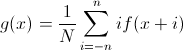thoughtlesslyjoyfully use it. Now let’s think, what is the physical meaning of derivatives in this place? We want to use them to determine the change in the value of a function in a finite neighborhood of a point, and the derivative gives an idea of ​​an infinitely small neighborhood. To expand this neighborhood, one could add a higher order of derivatives to the Taylor expansion, but this will lead to nonlinearities in the system, which will make it much more difficult to solve, and the advantages will be doubtful, especially since in practice we are not dealing with continuous, repeatedly differentiable functions, but with generally unclear what discrete functions. Therefore, it would be more logical to look for the function g (x), for which, in our discrete case, f (x) + g (x) = f (x + 1), f (x) + 2g (x) = f (x +2), f (x) - g (x) = f (x-1), and so on. Thus in this case, we need not a derivative, but a certain linear function that is closest to the points of the original function. Simple mathematical calculations lead to a solutionWhere 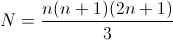. If we built the derivative on one neighboring point on each side, then we were lucky: in this case, the formula coincides with the formula for the approximate calculation of derivatives: g (x) = (f (x + 1) - f (x-1)) / 2. What is typical, in OpenCV, when calculating the optical flux of Lucas-Canada, this formula is used, we will come back to this later. But if you take more points, then the formula already becomes completely different from the classical difference schemes for the first derivative.

Obviously, if we build this function, for example, from three neighboring points to the left and to the right of the original one, then it does not depend on the points located farther in any way, and, accordingly, when shifting more than three points, we will often get inadequate results . And also, the greater the number of points on which we construct this function, the greater the average deviation of the resulting line from the points used - again, due to the fact that we do not have linearly changing images, but the devil knows which ones. In practice, shifts of more than 2 pixels already give an inadequately large error, no matter how many points we take.

Another weak point of the algorithm is that, again, we are dealing not with smooth continuous functions, but with arbitrary, and even discrete. Therefore, on some fragments of the image, the intensity can “jump” without any obvious regularities, for example, at the boundaries of objects, or due to noise. In this case, no function g (x) can accurately describe the image changes in the vicinity of the point. In order to overcome this (at least partially), it is proposed to smear the original image, and it will be useful to smear it quite strongly, that is, it is better to use not everyone’s favorite gaussian blur (averaging with weight coefficients), but just the same box filter (uniform averaging over the window ), and even several times in a row. Image smoothness is more important to us now than detail.

However, these measures also will not save us from limiting the detected shift of 2-3 pixels. And by the way, in OpenCV 1.0 there was such an implementation of the optical stream, and it worked only in ideal conditions at very small shifts.

What to do?

Total, ordinary Lucas-Canada well defines small shifts, such within which the picture is similar to its linear approximation. To overcome this, we will use the standard CV technique - multi-scaling: we will build a “pyramid” of images of different scales (it is almost always taken to scale 2 times on each axis, it’s easier to count) and go through them with an optical stream from a smaller image to a larger one then the detected small shift in the small image will correspond to the large shift in the large image. On the smallest image, we find a shift of no more than 1-2 pixels, and moving from a smaller scale to a larger one, we use the result from the previous step and refine the shift values. Actually, in OpenCV it is implemented by calcOptFlowPyrLK function. Using this pyramidal algorithm allows us not to bother with calculating a linear approximation at many points: it is easier to take more levels of the pyramid, and take a rather rough approximation of this function at each level. Therefore, in OpenCV and is calculated only two adjacent points. And therefore, in relation to this implementation of the algorithm, our conclusions about the advantage of the approximating function over the derivative turned out to be useless: for such a number of control points, the derivative is the best approximating function.

And what else are there?

This algorithm is not the only option for calculating the optical flux. In OpenCV, in addition to the Lucas-Canada stream, there is also the Farneback stream and SimpleFlow, also often refer to the Horn – Schunck algorithm.

Method Horn-Schunck is somewhat more global than the method of Lucas-Canada. It is based on the assumption that the optical flux throughout the image will be fairly smooth. It is proposed to move from the same equation to the functional , that is, add the requirement for the absence of a sharp change in the shifts with the weight coefficient α. Minimization of this functional leads us to a system of two equations:



In these equations, the Laplacians are proposed to calculate approximately:- the difference with the average value. We get a system of equations that we write for each pixel and solve the general system iteratively:



In this algorithm, it is also proposed to use multi-scaling, and it is recommended to scale images not by 2 times, but with a coefficient of 0.65.

This algorithm was implemented in the first versions of OpenCV, but later abandoned him.

Farneback proposed approximating the change in intensity in the neighborhood using a quadratic form: I = xAx + bx + c with a symmetric matrix A (in fact, considering the Taylor expansion to the first term, we took the linear approximation I = bx + c, that is, now we are like times decided to increase the accuracy of the approximation) If the image has shifted within this neighborhood, then, substitute into the quadratic expansion, open the brackets, we get


.

Now we can calculate the value of A, b, c of each image, and then the system will be redundant with respect to d (especially embarrassing first equation), and general d can be obtained from the second equation 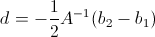. Necessary to resort to the following approximation: 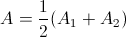. We also designate for simplicity 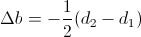. Then we obtain simply .

To compensate for the noise in the calculation, we again turn to the assumption that in the vicinity of the point under study, all points have more or less the same shift. Therefore, again, we integrate the error over the window with Gaussian weight coefficients w, and find the vector d minimizing this total error. Then we get the optimal value and the corresponding minimum error . That is, we need to calculate for each point , average over the window, invert the matrix and get the result. Accordingly, these products can be calculated for the whole picture and use pre-calculated values ​​for different points, that is, this is just the case when it makes sense to consider dense stream.

As usual, this algorithm has a number of modifications and improvements, primarily allowing the use of known a priori information - a given initial approximation of the flow - and, again, multi-scaling.

At the heart of the SimpleFlow methodthe following idea lies: if we still can not determine the shift more than the size of the window by which we searched for derivatives, then why bother with the calculation of derivatives? Let's just find the most similar point in the window! And to resolve ambiguities and to compensate for noise, we take into account that the flow is continuous and in the vicinity of this point all points have almost the same shift. And the problem with the window size is again solved by multi-scaling.

More precisely, the algorithm is as follows: for all points in the window is a function of the "energy" responsible (with inverse logarithmic dependence) for the transition probability is the starting point to this point: . Further, the convolution of this energy with a Gaussian window is consideredand the values ​​(dx, dy) are found that minimize this function. To obtain subpixel accuracy, we consider a small neighborhood of the found optimal point (dx, dy) and look for the peak of the energy function as the peak of a paraboloid in it. And, as mentioned above, this procedure is performed for the pyramid of scaled images. They also have cunning methods for speeding up calculations, but it’s interesting for everyone to figure it out themselves. It is important for us that due to this, this algorithm is (theoretically) quite fast with good accuracy. And he does not have such a problem as the previous ones, that the greater the shift, the worse it is detected.

And if you take not intensity?

It was said above that the correspondence between points can be determined by different quantities, so why do we consider only the intensity? And because any other value can be reduced to it: we simply filter the images with the appropriate filter and feed the filtered images to the input of the algorithms described above. Accordingly, if you want to use an optical stream, first think about which image characteristic will be the most stable under your conditions, and perform the appropriate filtering so that this characteristic is not the intensity at the input of the algorithm.

Practice

Let's try out in practice the algorithms that OpenCV offers us.

Here you can conduct a lot of different studies of each algorithm, varying the parameters, changing the input sequences - with different shifts, rotations, projective transformations, segments, with different noise, etc. This would take a lot of time and would exceed the size of the present article, therefore, I propose here to confine ourselves to the simple case of a parallel shift of the image by a fixed distance and the imposition of small noise. This will allow you to understand in general terms how to run the algorithms and which of them is cooler.

The syntax of the procedures is described in detail on the manual page , here I will give a squeeze-translation with my comments.

Classic Lucas-Canada is implemented with a pyramid in the calcOpticalFlowPyrLK procedure. The algorithm calculates the sparse stream, that is, for a given set of points in the first image, estimates their position in the second. The input parameters are quite obvious: two input images, the input and output sets of points, status - the output vector showing whether the corresponding point was found successfully, err - the output vector of estimated errors of the corresponding points, WinSize - the size of the window over which the Gaussian averaging occurs, I took 21x21 and it worked well, maxLevel - the number of layers in the pyramid minus one, that is, the number of the last layer, I took 5, criteria - the condition for exiting the iterative process of determining the shift (minimizing the error iteratively) - this I left the option by default, flags - optional flags, for example, you can use the initial approximation of the flow or choose a method for estimating the error, minEigThreshold - the threshold value of the gradient below which the matrix is ​​considered degenerate, I left it by default. Starting with OpenCV 2.4.1, you can use a pre-computed pyramid of scaled images to compute the stream.

The result of the work is that both small and large shifts are successfully and stably detected, resistant to fairly large noise, the operating time is about 10 ms for 400 points with a 5-layer pyramid (on core i7 950).

By the way, this algorithm is also implemented on Gpu (CUDA), both dense and sparse versions.

The Farneback stream is implemented by the calcOpticalFlowFarneback procedure, the dense stream is calculated, that is, the shift of each point. Parameters: input images, output stream in the format of a two-channel matrix of floats, pyr_scale determines the ratio of the scales between the layers of the pyramid, levels - the number of levels in the pyramid, winsize - the size of the window to be averaged, iterations - the number of iterations at each level, poly_n - the size of the polynomial by which the values ​​of A and b are estimated, poly_sigma is the sigma of the Gaussian blur when smoothing the derivatives, the recommended parameter values ​​are indicated in the manual, flags are additional flags, for example, you can use the initial approximation ix flow or otherwise averaged over the window.

This algorithm is much less stable (according to my observations), it is easier to miss on fairly uniform pictures (apparently, the problem is the lack of filtering of unsuccessful points), poorly determines large shifts. I worked for 600 ms on a 512x512 image.

The SimpleFlow stream implements the calcOpticalFlowSF procedure (the dense stream is calculated again), and it has many mysterious parameters without default values, and in general, at the moment, the information on the page is very concise. Let's try to figure it out. The first 3 are input images and output two-channel; layers - the number of layers in the pyramid, that is, how many times the original image is scaled; averaging_block_size - the size of the window in which we calculated the pixel energy function; max_flow - the maximum shift that we want to be able to determine at each step, in fact it is determined by the size of the window (although it is not entirely clear why it is int). You can stop here, or you can set a few more parameters, the meaning of some of them eludes me.

The site offers to see an exampleits use, in which it starts with the following parameters: calcOpticalFlowSF (frame1, frame2, flow, 3, 2, 4, 4.1, 25.5, 18, 55.0, 25.5, 0.35, 18, 55.0, 25.5, 10);

My algorithm works much slower than others, about 9-12 seconds per 512x512 picture. The result of the work seems more plausible than Farneback, at least the shift in uniform pictures is better defined, it works much better with large shifts.

conclusions

If you want to use the optical stream somewhere, first think about whether you need it: you can often do with simpler methods. To undertake to implement the flow yourself is worth only a few times thinking: each algorithm has many tricks, subtleties and optimizations; no matter what you do, most likely it works better in OpenCV (naturally, provided that it is there). Moreover, they use logical and hardware optimizations there, such as using SSE instructions, multithreading, the ability to calculate with CUDA or OpenCL, etc. If you just need to calculate the shift of a certain set of points (i.e. sparse stream), you can safely use function calcOpticalFlowPyrLK, it works well, reliable and fast enough. It is good to use calcOpticalFlowSF function to calculate dense-stream. but it works very slowly. If performance is critical, then calcOpticalFlowFarneback, but you still need to make sure that the results of its work will suit you.

Literature

docs.opencv.org/modules/video/doc/motion_analysis_and_object_tracking.html
Pyramidal Implementation of the Lucas Kanade Feature Tracker. Description of the algorithm - Jean-Yves Bouguet
Two-Frame Motion Estimation Based on Polynomial Expansion - Gunnar Farneback
SimpleFlow: A Non-iterative, Sublinear Optical Flow Algorithm - Michael Tao, Jiamin Bai, Pushmeet Kohli, and Sylvain Paris
Horn-Schunck Optical Flow with a Multi-Scale Strategy - Enric Meinhardt-Llopis, Javier Sanchez
en.wikipedia.org/wiki/Optical_flow