Visualization of a two-dimensional Gaussian in the plane

Good day. In the process of developing one of the clustering methods, I had a need to visualize a Gaussian (draw an ellipse in fact) on a plane along a given covariance matrix . But somehow, I didn’t immediately think that behind a simple drawing of a regular ellipse by 4 numbers, there were some difficulties. It turned out that the calculation of the ellipse points using eigenvalues and eigenvectors of the covariance matrix, the Mahalanobis distance , as well as quantile of chi-square distribution , which I, frankly, did not use to the university is never.

Data and their relative position

Let's start with the initial conditions. So, we have some array of two-dimensional data

for which we can easily find out the covariance matrix and average values ​​(center of the future ellipse):

plot(data[, 1], data[, 2], pch=19, asp=1, 
     col=rgb(0, 0.5, 1, 0.2),
     xlab="x", ylab="y")
sigma <- cov(data)
m.x <- mean(data[, 1])
m.y <- mean(data[, 2])

Before you start drawing an ellipse, you need to decide what size the shape will be. Here are some examples:

To determine the size of the ellipse, recall the Mahalanobis distance between two random vectors from the same probability distribution with the covariance matrix Σ :



You can also determine the distance from the random vector x to the set with the average value μ and the covariance matrix Σ :



It is worth noting that in the case when Σequal to the identity matrix, the Mahalanobis distance degenerates into the Euclidean distance. The meaning of the Mahalanobis distance is that it takes into account the correlation between the variables; or in other words, the spread of data relative to the center of mass is taken into account (it is assumed that the spread is in the form of an ellipsoid). In the case of using the Euclidean distance, the assumption is used that the data are distributed spherically (evenly across all measurements) around the center of mass. We illustrate this by the following graph: The

center of mass is marked in yellow, and the two red points from the dataset located on the main axes of the ellipse are at the same (in the sense of Mahalanobis) distance from the center of mass.

Ellipse and chi-square distribution

An ellipse is a central non-degenerate second-order curve, its equation can be written in general form (we will not write down restrictions):



On the other hand, we can write the ellipse equation in matrix form (in homogeneous two-dimensional coordinates):



and obtain the following expression, in order to show that an ellipse is really given in matrix form:



Now let's recall the distance of Mahalanobis and consider its square:



It is easy to notice that this representation is identical to writing the ellipse equation in matrix form. Thus, we were convinced that the Mahalanobis distance describes an ellipse in Euclidean space. The Mahalanobis distance is simply the distance between a given point and the center of mass divided by the width of the ellipsoid in the direction of the given point.

A delicate moment comes to understand, it took me some time to realize: the square of the Mahalanobis distance is the sum of the squares of the kth number of normally distributed random variables , where n is the dimension of space.

Recall that such a chi-square distribution is a distribution of the sum of squares of k independent standard normal random variables (this distribution is parameterized by the number of degrees of freedom k). And this is precisely the distance of Mahalanobis. Thus, the probability that x is inside the ellipse is expressed by the following formula:



And here we come to the answer to the question about the size of the ellipse - we will determine its size by quantiles chi-square distribution, this is easily done in R (where q is from (0, 1) and k is the number of degrees of freedom):

v <- qchisq(q, k)

Getting an ellipse path

The idea of ​​generating the contour of the ellipse we need is very simple, we just take a number of points on the unit circle, shift this circle to the center of mass of the data array, then scale and stretch this circle in the desired directions. Consider the geometric interpretation of the multidimensional Gaussian distribution: as we know, this is an ellipsoid, in which the direction of the main axes is given by the eigenvalues ​​of the covariance matrix, and the relative length of the main axes is given by the root of the corresponding eigenvalues.

The following graph shows the eigenvectors of the covariance matrix scaled to the roots of the corresponding eigenvalues, the directions correspond to the main axes of the ellipse:



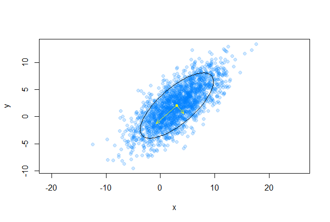
Consider the expansion of the covariance matrix in the following form:



where UIs the matrix formed by the unit eigenvectors of the matrix Σ , and Λ is the diagonal matrix made up of the corresponding eigenvalues.

e <- eigen(sigma)

And also consider the following expression for a random vector from a multidimensional normal distribution:



Thus, the distribution N (μ, Σ) is, in fact, the standard multidimensional normal distribution N (0, I) scaled by Λ ^ (1/2) , rotated on U and shifted by μ .

Let's now write a function that draws an ellipse with the following input:

• mx, my - coordinates of the center of mass
• sigma - covariance matrix
• q is the quantile of the chi-square distribution
• n - ellipse sampling density (the number of points on which the ellipse will be built)

GetEllipsePoints <- function(m.x, m.y, sigma, q = 0.75, n = 100)
{
  k <- qchisq(q, 2) # вычисляем значение квантиля
  sigma <- k * sigma # масштабирование ковариационной матрицы на значение квантиля
  e <- eigen(sigma) # вычисление собственных значений масштабированной ковариационной матрицы
  angles <- seq(0, 2*pi, length.out=n) # разбиваем круг на n-ое количество углов
  cir1.points <- rbind(cos(angles), sin(angles)) # генерируем точки на единичной окружности
  ellipse.centered <- (e$vectors %*% diag(sqrt(abs(e$values)))) %*% cir1.points # масштабируем и поворачиваем полученный датасет
  ellipse.biased <- ellipse.centered + c(m.x, m.y) # смещаем его до центра масс
  return(ellipse.biased) # готово
}

Result

The following code draws many confidence ellipses around the dataset's center of mass:

points(m.x, m.y, pch=20, col="yellow")
q <- seq(0.1, 0.95, length.out=10)
palette <- cm.colors(length(q))
for(i in 1:length(q))
{
  p <- GetEllipsePoints(m.x, m.y, sigma, q = q[i])
  points(p[1, ], p[2, ], type="l", col=palette[i])
}
e <- eigen(sigma)
v <- (e$vectors %*% diag(sqrt(abs(e$values))))
arrows(c(m.x, m.x), c(m.y, m.y), 
       c(v[1, 1] + m.x, v[1, 2] + m.x), c(v[2, 1] + m.y, v[2, 2] + m.y), 

As a result, we get the following picture:

Read

• Gaussians
• Some notes on ellipses

The code can be found on my github .