Mask R-CNN: Modern Neural Network Architecture for the Segmentation of Objects in Images

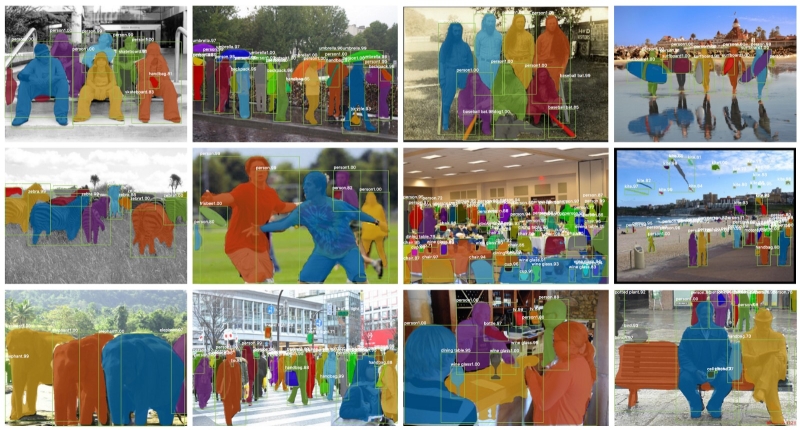
The times when one of the most urgent tasks of computer vision was the ability to distinguish pictures of dogs from pictures of cats, are already in the past. At the moment, neural networks are able to perform much more complex and interesting tasks on image processing. In particular, the network with the Mask R-CNN architecture makes it possible to select the outlines (“masks”) of different objects in photographs, even if there are several such instances, they have different sizes and partially overlap. The network is also capable of recognizing the poses of people in an image.

Earlier this year I had the opportunity to participate in the Data Science Bowl 2018 competition at Kaggle for educational purposes. For educational purposes, I used one of those models that generously spread by some participants in high positions. It was a neural network with the Mask R-CNN architecture, recently developed by Facebook Research. (It is worth noting that the winning team still used a different architecture - U-Net. Apparently, more suitable for biomedical tasks, to which the Data Science Bowl 2018 belonged).
Since the goal was to familiarize ourselves with the tasks of Deep Learning, and not to occupy a high place, after the end of the competition, there was a strong desire to understand how the used neural network was “under the hood”. This article presents a summary of information obtained from the original documents from arXiv.org and several articles on Medium. The material is purely theoretical in nature (although at the end there are references about practical use), and it does not contain more than it has in the indicated sources. But there is little information on the topic in Russian, so perhaps the article will be useful to someone.

All illustrations are from foreign sources and belong to their rightful owners.

Computer vision task types

Usually, modern computer vision tasks are divided into four types (there were no translations of their names even in Russian-language sources, therefore in English, so as not to create confusion):

• Classification - image classification by the type of object it contains;
• Semantic segmentation - the definition of all pixels of objects of a particular class or background in the image. If several objects of the same class overlap, their pixels are not separated from each other;
• Object detection - detection of all objects of the specified classes and definition of the covering frame for each of them;
• Instance segmentation - the definition of the pixels belonging to each object of each class separately;

On the example of the image with balloons from [9], this can be illustrated as follows:

Evolutionary Development Mask R-CNN

The concepts underlying the Mask R-CNN have undergone a phased development through the architectures of several intermediate neural networks that solved different tasks from the list above. Probably the easiest way to understand the principles of the functioning of this network is to consistently consider all these stages.

Without dwelling on basic things like back propagation, non-linear activation functions, and what the multilayer neural network in general is like, briefly explain how the layers of Convolution Neural Networks work are probably worth it (R-CNN).

Convolution and MaxPooling

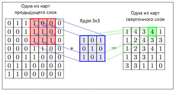
The convolutional layer allows you to combine the values ​​of adjacent pixels and highlight the more general features of the image. To do this, in the picture consistently slide a square window of a small size (3x3, 5x5, 7x7 pixels, etc.) called the kernel. Each core element has its own weight multiplied by the value of the image pixel on which the core element is currently superimposed. Then the numbers obtained for the whole window are added together, and this weighted sum gives the value of the next attribute.

To obtain the matrix ("maps") of the features of the entire image, the core is sequentially shifted horizontally and vertically. In the next layers, the convolution operation is applied already to feature maps obtained from the previous layers. Graphically, the process can be illustrated as follows:



An image or feature maps within a single layer can be scanned not by one, but by several independent filters, thus giving not only one map to output, but several (they are also called “channels”). Setting the weights of each filter is done using the same backpropagation procedure.

Obviously, if the filter core does not go beyond the image when scanning, the dimension of the feature map will be less than the original image. If you want to keep the same size, apply the so-called paddings - the values ​​that complement the image along the edges and which are then captured by the filter along with the actual pixels of the image.


In addition to paddings, strides also affect the dimension change - the step values ​​with which the window is moved around the image / map.

Convolution is not the only way to obtain a generalized characteristic of a group of pixels. The easiest way to do this is to select one pixel by a given rule, for example, the maximum one. This is exactly what the MaxPooling layer does.


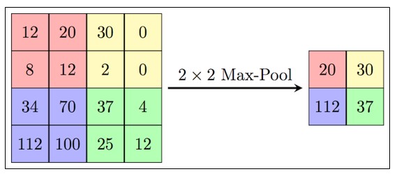
Unlike convolution, maxpooling is usually applied to non-intersecting groups of pixels.

R-CNN

The R-CNN (Regions With CNNs) network architecture was developed by a team from UC Berkley to apply Convolution Neural Networks to the object detection task. The approaches to solving such problems that existed at that time approached the maximum of their capabilities and did not significantly improve their performance.

CNN did well in classifying images, and on this network they were essentially applied to the same. For this purpose, not all of the entire image was submitted to the CNN input, but regions previously pre-allocated in another way, which presumably contained some objects. At that time there were several such approaches, the authors chose Selective Search , although they indicate that there are no particular reasons for choosing it.

As a CNN network, a ready-made architecture was also used - CaffeNet (AlexNet). Such neural networks, like the others for the ImageNet image set, are classified into 1000 classes. R-CNN was developed to detect objects of a smaller number of classes (N = 20 or 200), so the last CaffeNet classification layer was replaced with a layer with N + 1 outputs (with an additional background class).

Selective Search yielded about 2000 regions of different sizes and aspect ratios, but CaffeNet takes as input the images of a fixed size of 227x227 pixels, so before submitting the regions to the network input they had to be modified. For this, the image from the region was enclosed in the smallest covering square. Along the (lesser) side along which the fields were formed, several “contextual” (surrounding the region) image pixels were added, the rest of the field was not filled with anything. The resulting square was scaled to size 227x227 and fed to the input of CaffeNet.


Despite the fact that CNN trained to recognize the N + 1 classes, in the end it was used only to extract a fixed 4096-dimensional feature vector. N linear SVMs were engaged in the direct determination of the object in the image, each of which carried out a binary classification according to its type of objects, determining whether there is one in the transferred region or not. In the original document, the whole procedure is illustrated by the following scheme:


The authors argue that the classification process in SVM is very productive, representing in essence just matrix operations. Characteristic vectors obtained from CNN are combined across all regions into a 2000x4096 matrix, which is then multiplied by a 4096xN matrix with SVM weights.

It should be noted that regions obtained with the help of Selective Search can only contain some objects, and not the fact that they contain all of them. Whether a region is considered to contain an object or not is determined by the Intersection over Union (IoU) metric. This metric is the ratio of the area of ​​intersection of a rectangular candidate region with a rectangle, actually embracing the object, to the area of ​​the union of these rectangles. If the ratio exceeds a specified threshold, the candidate region is considered to contain the desired object.

IoU was also used to screen out an excessive amount of regions containing a specific object (non-maximum suppression). If the IoU of a certain region with a region that received the maximum result for the same object was above a certain threshold, the first region was simply discarded.

In the course of the error analysis procedure, the authors also developed a method to reduce the error in highlighting the enclosing frame of the object - the bounding-box regression. After classifying the contents of the candidate region, using the linear regression based on the characteristics of CNN, four parameters were determined - (dx, dy, dw, dh). They described how much it is necessary to shift the center of the region's frame in x and y, as well as how much to change its width and height in order to more accurately cover the recognized object.

Thus, the procedure for detecting objects by the R-CNN network can be divided into the following steps:

1. Selection of candidate regions with the help of selective search.
2. Conversion of the region to the size taken by CNN CaffeNet.
3. Receiving using CNN 4096-dimensional feature vector.
4. Conduct N binary classifications of each feature vector using N linear SVMs.
5. Linear regression of region frame parameters for more accurate coverage of the object

The authors noted that the architecture developed by them also showed itself well in the semantic segmentation task.

Fast R-CNN

Despite good results, the performance of R-CNN was still low, especially for deeper than CaffeNet networks (such as VGG16). In addition, learning the bounding box regressor and SVM required saving a large number of features to disk, so it was expensive in terms of storage size.

The authors of Fast R-CNN proposed to speed up the process at the expense of a couple of modifications:

• Pass through CNN not each of the 2,000 candidate regions individually, but the entire image. The proposed regions are then superimposed on the resulting common feature map;
• Instead of independent training of three models (CNN, SVM, bbox regressor), combine all the training procedures into one.

The conversion of features that fell into different regions to a fixed size was performed using the RoIPooling procedure . A region window of width w and height h is divided into a grid having H × W cells of size h / H × w / W. (The authors of the document used W = H = 7). Max Pooling was performed for each such cell to select only one value, thus giving the resulting H × W trait matrix.

Binary SVMs were not used, instead, selected features were transferred to a fully connected layer, and then to two parallel layers: softmax with K + 1 outputs (one for each class + 1 for the background) and a bounding box regressor.

The overall network architecture looks like this:


For joint training of the softmax classifier and bbox regressor, a combined loss function was used:

$$

Here:
$$ - class of the object actually depicted in the candidate region;
$$ - log loss for class u;
$$ - real changes in the scope of the region for more accurate coverage of the object;
$$ - predicted changes in the scope of the region;
$$ - loss-function between the predicted and real changes in the frame;
$$ - indicator function equal to 1 when $$, and 0, when vice versa. By class$$ denotes the background (i.e., the absence of objects in the region).
$$- coefficient intended to balance the contribution of both loss functions to the overall result. In all experiments of the authors of the document, however, it was equal to 1.

The authors also mention that in order to speed up the calculations in the fully connected layer, they used the decomposition of the weights matrix according to Truncated SVD.

Faster R-CNN

After the improvements made in Fast R-CNN, the mechanism for generating candidate regions turned out to be the bottleneck of the neural network. In 2015, a team from Microsoft Research was able to make this stage much faster. They offered to calculate the regions not by the original image, but again by the map of the signs obtained from CNN. For this, a module has been added called Region Proposal Network (RPN). The new architecture is as follows:


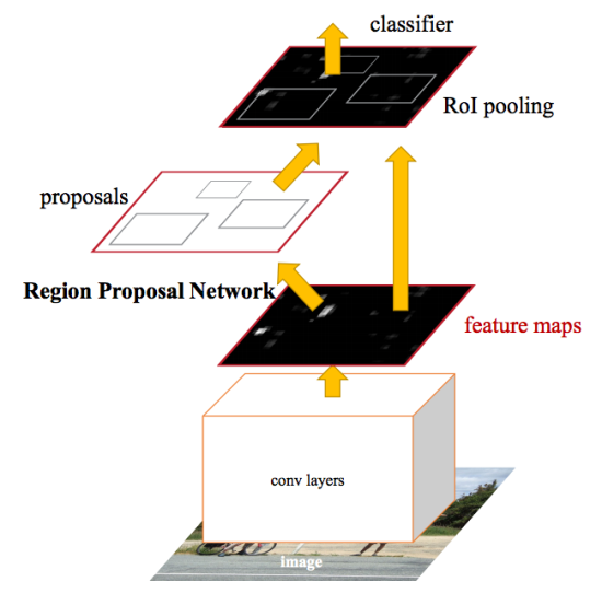
As part of the RPN, according to the extracted CNN features, they slide along a “mini-neural network” with a small (3x3) window. The values ​​obtained with its help are transmitted in two parallel fully connected layers: the box-regression layer (reg) and the box-classification layer (cls). The outputs of these layers are based on the so-called anchor-ah: k framework for each position of the sliding window, having different sizes and aspect ratios. The reg-layer for each such anchor produces 4 coordinates each, correcting the position of the enclosing frame; The cls-layer produces two numbers each - the probability that the frame contains at least some object or that does not contain. The document illustrates this pattern:


The learning process of reg and cls layers is combined; loss function they have a common, representing the sum of the loss functions of each of them, with a balancing coefficient.

Both RPN layers issue only offers for candidate regions. Those that have a high probability of containing any object are transmitted further to the object detection module and the refinement of the covering frame, which is still implemented as Fast R-CNN.

In order to share the characteristics obtained in CNN between the RPN and the detection module, the learning process of the entire network is built iteratively, using several steps:

1. Initialized and trained to identify candidate regions RPN-part.
2. Using the proposed RPN regions, the Fast R-CNN part is re-trained.
3. A trained detection network is used to initialize weights for the RPN. Common convolution layers, however, are captured and only RPN-specific layers are configured.
4. With fixed convolution layers, Fast R-CNN is finally tuned up.

The proposed scheme is not unique, and even in its current form it can be continued with further iterative steps, but the authors of the original research conducted experiments exactly after such training.

Mask R-CNN

Mask R-CNN develops the Faster R-CNN architecture by adding another branch that predicts the position of the mask covering the found object, and thus solves the problem of instance segmentation. A mask is simply a rectangular matrix in which 1 at some position means that the corresponding pixel belongs to an object of a given class, 0 means that the pixel does not belong to the object.



Colorful masks can be rendered on the source images with colorful images:



The authors of the document conventionally share the developed architecture on the CNN network for computing image attributes, called the backbone, and head combining the parts responsible for predicting the enclosing frame, classifying the object and determining its mask. Loss function for them is common and includes three components:

$$

The selection of the mask occurs in the class-agnostic style: the masks are predicted separately for each class, without prior knowledge of what is depicted in the region, and then the mask of the class that won the independent classifier is simply selected. It is argued that this approach is more effective than relying on a priori knowledge of the class.

One of the main modifications that arose because of the need to predict a mask is a change in the RoIPool procedure (calculating a matrix of attributes for a candidate region) to a so-called RoIAlign. The fact is that the feature map obtained from CNN is smaller than the original image, and a region covering an integer number of pixels on an image cannot be displayed in a proportional region of a map with an integer number of features:




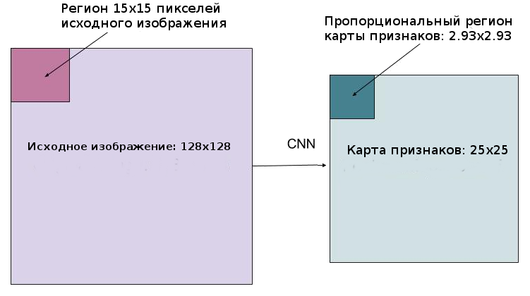
In RoIPool, the problem was solved simply by rounding the fractional values ​​to integers. This approach works fine when highlighting a spanning frame, but the mask calculated on the basis of such data is too inaccurate.

In contrast, rounding is not used in RoIAlign, all numbers remain valid, and bilinear interpolation at the four nearest integer points is used to calculate feature values.

In the original document, the difference is explained as follows:


Here, the feature map is marked with a dashed grid, and a continuous map displays the signs of the candidate region from the source photo. 4 groups for max pooling with 4 signs indicated by dots in the figure should fall into this region. Unlike the RoIPool procedure, which, due to rounding, would simply align the region with integer coordinates, RoIAlign leaves points in their current locations, but calculates the values ​​of each of them using bilinear interpolation using the four nearest features.


In addition to the high results in the tasks of instance segmentation and object detection, the Mask R-CNN turned out to be suitable for determining the poses of people in the photograph (human pose estimation). The key point here is the selection of reference points (keypoints), such as the left shoulder, right elbow, right knee, etc., which can be used to draw the skeleton of a person’s position:



To determine the control points, the neural network is trained in such a way that it gives out masks which only one pixel (the same point) had a value of 1, and the rest - 0 (one-hot mask). At the same time, the network is trained to issue K such single-pixel masks, one for each type of reference point.

Feature Pyramid Networks

In the experiments on the Mask R-CNN, along with the usual CNN ResNet-50/101 as a backbone, the feasibility of using the Feature Pyramid Network (FPN) was also conducted. They showed that the use of FPN in the backbone gives the Mask R-CNN an increase in both accuracy and performance. This makes a useful description of this improvement, in spite of the fact that a separate document is dedicated to it and it is little connected with the series of articles under consideration.
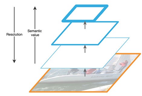
The purpose of the Feature Pyramids, like image pyramids, is to improve the quality of detection of objects, taking into account the large range of their possible sizes.

Feature Pyramid Network feature maps, extracted by successive layers of CNN with decreasing dimension, are considered as a kind of hierarchical “pyramid” called the bottom-up pathway. At the same time, the feature maps of the lower and upper levels of the pyramid have their own advantages and disadvantages: the first have high resolution, but low semantic, generalizing ability; the second - on the contrary:


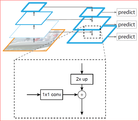
The FPN architecture allows you to combine the advantages of upper and lower layers by adding top-down pathway and lateral connections. For this, the map of each overlying layer increases to the size of the underlying layer and their contents are elementwise added. The final predictions use result maps of all levels.

Schematically, this can be represented as:


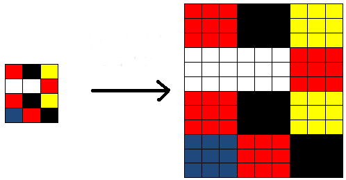
Increasing the size of the top-level map (upsampling) is done by the simplest method - the nearest neighbor, i.e., something like this:

useful links

Original research papers on arXiv.org:

1. R-CNN: https://arxiv.org/abs/1311.2524

2. Fast R-CNN: https://arxiv.org/abs/1504.08083

3. Faster R-CNN : https://arxiv.org/abs/1506.01497

4. R-CNN Mask: https://arxiv.org/abs/1703.06870

5. Feature Pyramid Network: https://arxiv.org/abs/1612.03144

On medium. com on Mask R-CNN is a lot of articles, they are easy to find. I cite only those that I have read as references:

6. Simple Understanding of Mask RCNN - a summary of the principles of the resulting architecture.

7. A Brief History of CNNs in Image Segmentation: From R-CNN to Mask R-CNN- The history of the network in the same chronological order as in this article.

8. From R-CNN to Mask R-CNN is another consideration of the stages of development.

9.R-CNN and TensorFlow Splash of Color: Instance Segmentation with Mask is a neural network implementation in the Matterport Opensource library.

The last article, in addition to describing the principles of Mask R-CNN, offers the opportunity to try the network in practice: for coloring balloons with different colors on black and white images.

In addition, you can practice with the neural network on the model that I used in the kaggle Data Science Bowl 2018 competition (but not only with this model, of course; you can find a lot of interesting things in the Kernels and Discussions sections):

10. Mask R- CNN in PyTorch by Heng CherKeng. The implementation involves a number of steps for deployment, the author provides instructions. The model requires PyTorch 0.4.0, support for GPU computing, NVIDIA CUDA. If my own system does not meet the requirements, I can recommend Amazon AMI Deep Virtual Learning images (Amazon instances are paid, with hourly billing, the minimum suitable size, apparently, is p2.xlarge).

I also came across here, in Habré, an article about using the network from Matterport in processing images with dishes (but without source codes). Hopefully, the author will only be happy for an additional mention:

11. ConvNets. Project prototyping using R-CNN Mask