Introduction to Algorithm Complexity Analysis (Part 4)
- Transfer
- Tutorial
From the translator: this text is given with minor abbreviations due to places of excessive "chewed up" material. The author absolutely rightly warns that certain topics may seem too simple or well-known to the reader. Nevertheless, to me personally this text helped to streamline the existing knowledge on the analysis of the complexity of algorithms. I hope that it will be useful to someone else.
Due to the large volume of the original article, I broke it into parts, of which there will be a total of four.
I (as always) will be extremely grateful for any comments in PM on improving the quality of translation.
Published earlier:
Part 1
Part 2
Part 3
Congratulations! Now you know how to analyze the complexity of algorithms, what is the asymptotic estimate and the notation “big-O”. You also know how to intuitively figure out whether the algorithm complexity
This final section is optional. It’s a bit more complicated, so you can feel free to skip it if you want. You will need to focus and spend some time solving exercises. However, as will be shown here is a very useful and powerful way to analyze the complexity of algorithms, which, of course, art of attention to IT.
We looked at a sorting implementation called selection sorting, and mentioned that it is not optimal. The optimal algorithm is the one that solves the problem in the best way, implying that there is no algorithm that does this better. Those. all other algorithms for solving this problem have the same or used formore difficulty. There may be a ton of optimal algorithms having the same complexity. The same sorting problem can be solved optimally in many ways. For example, we can use the same idea for quick sorting as in binary search. This method is called merge sort .
Before we implement the actual merge sort, we need to write an auxiliary function.
The function
An analysis of this algorithm shows that its execution time is
Using this function, we can build a better sorting algorithm. The idea is this: we split the array into two parts, recursively sort each of them and combine the two sorted arrays into one. Pseudocode:
This feature is harder to understand than the previous ones, so the next exercise may take you longer.
As a final exercise, let's analyze the difficulty
So, we split the original array into two parts,
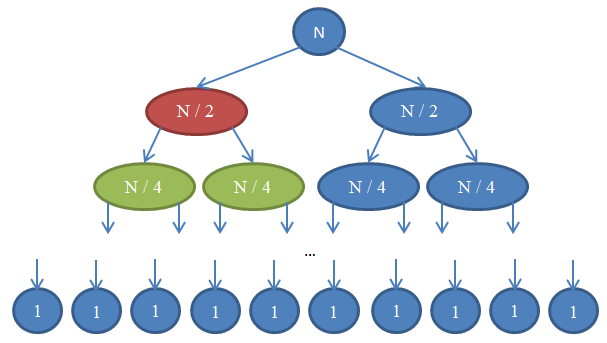
Let's see what happens here. Each circle represents a function call.
Note that the number of elements in each row remains the same.
As a result, the complexity of each line is
As you saw in the last example, complexity analysis allows us to compare algorithms to figure out which one is better. Based on these considerations, we can now be sure that for large-sized arrays, merge sorting is far ahead of selection sorting. Such a conclusion would be problematic if we did not have a theoretical basis for the analysis of the algorithms we developed. Undoubtedly, runtime sorting algorithms are
After studying this article, your intuition about analyzing the complexity of algorithms should help you create fast programs and focus your optimization efforts on those things that really have a big impact on the speed of execution. All together will allow you to work more productively. In addition, the mathematical language and notations (for example, “big O”) discussed in this article will be useful for you when communicating with other software developers when it comes to runtime algorithms, and I hope you can put into practice the acquired knowledge.
This article is published under the Creative Commons 3.0 Attribution . This means that you can copy it, publish it on your websites, make changes to the text, and generally do whatever you like with it. Just do not forget to mention my name. The only thing: if you base your work on this text, I urge you to publish it under Creative Commons to facilitate collaboration and the dissemination of information.
Thank you for reading to the end!
Due to the large volume of the original article, I broke it into parts, of which there will be a total of four.
I (as always) will be extremely grateful for any comments in PM on improving the quality of translation.
Published earlier:
Part 1
Part 2
Part 3
Optimal sorting
Congratulations! Now you know how to analyze the complexity of algorithms, what is the asymptotic estimate and the notation “big-O”. You also know how to intuitively figure out whether the algorithm complexity
O( 1 ), O( log( n ) ), O( n ), O( n2 ) , and so on. Are you familiar with the symbols o, O, ω, Ω, Θand the concept of "worst case". If you get to this place, then my article has already completed its task.This final section is optional. It’s a bit more complicated, so you can feel free to skip it if you want. You will need to focus and spend some time solving exercises. However, as will be shown here is a very useful and powerful way to analyze the complexity of algorithms, which, of course, art of attention to IT.
We looked at a sorting implementation called selection sorting, and mentioned that it is not optimal. The optimal algorithm is the one that solves the problem in the best way, implying that there is no algorithm that does this better. Those. all other algorithms for solving this problem have the same or used formore difficulty. There may be a ton of optimal algorithms having the same complexity. The same sorting problem can be solved optimally in many ways. For example, we can use the same idea for quick sorting as in binary search. This method is called merge sort .
Before we implement the actual merge sort, we need to write an auxiliary function.
mergeLet's call it , and let it take two already sorted arrays and combine them into one (also sorted). This is easy to do:def merge( A, B ):
if empty( A ):
return B
if empty( B ):
return A
if A[ 0 ] < B[ 0 ]:
return concat( A[ 0 ], merge( A[ 1...A_n ], B ) )
else:
return concat( B[ 0 ], merge( A, B[ 1...B_n ] ) )
The function
concattakes an element (“head”) and an array (“tail”) and connects them, returning a new array with a “head” as the first element and a “tail” as the remaining elements. For example, concat( 3, [ 4, 5, 6 ] )will return [ 3, 4, 5, 6 ]. We use A_nand B_nto denote the sizes of arrays Aand Brespectively.Exercise 8
Make sure the function above actually does the merge. Rewrite it in your favorite programming language using iterations (for loop) instead of recursion.
An analysis of this algorithm shows that its execution time is
Θ( n ), where nis the length of the resulting array ( n = A_n + B_n).Exercise 9
Check what the runtime
mergeis Θ( n ).Using this function, we can build a better sorting algorithm. The idea is this: we split the array into two parts, recursively sort each of them and combine the two sorted arrays into one. Pseudocode:
def mergeSort( A, n ):
    if n = 1:
        return A # it is already sorted
    middle = floor( n / 2 )
    leftHalf = A[ 1...middle ]
    rightHalf = A[ ( middle + 1 )...n ]
    return merge( mergeSort( leftHalf, middle ), mergeSort( rightHalf, n - middle ) )
This feature is harder to understand than the previous ones, so the next exercise may take you longer.
Exercise 10
Make sure
mergeSortthat it is correct (i.e. check that it correctly sorts the array passed to it). If you cannot understand why it basically works, then manually solve a small example. At the same time, do not forget to make sure that leftHalfthey rightHalfare obtained when the array is split in half. A partition does not have to be exactly in the middle if, for example, an array contains an odd number of elements (this is what we need the function for floor).As a final exercise, let's analyze the difficulty
mergeSort. At each step, we split the original array into two equal parts (similarly binarySearch). However, in this case further calculations occur on both parts. After the recursion returns, we apply the operation to the results merge, which takes Θ( n )time. So, we split the original array into two parts,
n / 2each sized . When we connect them, the nelements will participate in the operation , therefore, the execution time will be Θ( n ). The figure below explains this recursion: Let's see what happens here. Each circle represents a function call.
mergeSort. The number in the circle indicates the number of elements in the array to be sorted. The top blue circle is the initial call mergeSortfor an array of size n. Arrows show recursive calls between functions. The original call mergeSortspawns two new ones for arrays, n / 2each sized . In turn, each of them generates two more calls with arrays in n / 4elements, and so on until we get an array of size 1. This diagram is called a recursive tree because it illustrates the operation of recursion and looks like a tree (more precisely, how inversion of a tree with a root above and leaves below). Note that the number of elements in each row remains the same.
n. Also note that each calling node uses the mergeresults from the called nodes for the operation . For example, a red node sorts n / 2items. To do this, it splits the n / 2array into two by n / 4, recursively calls with each of them mergeSort(green nodes) and combines the results into a single whole size n / 2. As a result, the complexity of each line is
Θ( n ). We know that the number of such rows, called the depth of the recursive tree, will be log( n ). The reason for this is the same arguments that we used for binary search. So, we have log( n )lines to the complexity Θ( n ), therefore, the overall complexity mergeSort: Θ( n * log( n ) ). It is much better thanΘ( n2 ) , which gives us sorting by choice (remember, log( n )much less n, so n * log( n )also much less than n * n = n2 ). As you saw in the last example, complexity analysis allows us to compare algorithms to figure out which one is better. Based on these considerations, we can now be sure that for large-sized arrays, merge sorting is far ahead of selection sorting. Such a conclusion would be problematic if we did not have a theoretical basis for the analysis of the algorithms we developed. Undoubtedly, runtime sorting algorithms are
Θ( n * log( n ) )widely used in practice. For example, the Linux kernel uses an algorithm called heap sorting., which has the same runtime as merge sort. Note that we will not prove the optimality of these sorting algorithms. This would require much more cumbersome mathematical arguments, but be sure: from the point of view of complexity, you can not find a better option.After studying this article, your intuition about analyzing the complexity of algorithms should help you create fast programs and focus your optimization efforts on those things that really have a big impact on the speed of execution. All together will allow you to work more productively. In addition, the mathematical language and notations (for example, “big O”) discussed in this article will be useful for you when communicating with other software developers when it comes to runtime algorithms, and I hope you can put into practice the acquired knowledge.
Instead of a conclusion
This article is published under the Creative Commons 3.0 Attribution . This means that you can copy it, publish it on your websites, make changes to the text, and generally do whatever you like with it. Just do not forget to mention my name. The only thing: if you base your work on this text, I urge you to publish it under Creative Commons to facilitate collaboration and the dissemination of information.
Thank you for reading to the end!
References
- Cormen, Leiserson, Rivest, Stein. Introduction to Algorithms , MIT Press
- Dasgupta, Papadimitriou, Vazirani. Algorithms , McGraw-Hill Press
- Fotakis. Course of Discrete Mathematics at the National Technical University of Athens
- Fotakis. Course of Algorithms and Complexity at the National Technical University of Athens