Network for the most experienced. Part fifteen. QoS
- Tutorial
СДСМ-15. About QoS. Now with the ability to pull requests .
And here we come to the topic of QoS.
Do you know why only now and why this will be the closing article of the entire course of SDCM? Because QoS is unusually complex. The hardest thing that was previously in the cycle.
This is not some kind of magic archiver, which will cleverly compress traffic on the fly and push your gigabit into a one-megabyte uplink. QoS is about how to sacrifice something unnecessary, cramming nevpihuemoe within the limits of what is permitted.
QoS is so enmeshed with the aura of shamanism and inaccessibility that all young (and not only) engineers try to carefully ignore its existence, believing that it is enough to shower problems with money and endlessly expanding links. True, until they realize that with such an approach, failure inevitably awaits them. Either the business will start asking uncomfortable questions, or there will be a lot of problems almost unrelated to the width of the channel, but directly dependent on the effectiveness of its use. Yeah, VoIP is actively waving a handle from behind the scenes, and multicast traffic sarcastically strokes your back.
Therefore, let's just realize that QoS is necessary, it will have to get to know one way or another, and why not start now in a calm atmosphere.
1. What determines QoS?
2. Three QoS models
3. DiffServ mechanisms
4. Classification and labeling
5. Queues
6. Congestion Avoidance
7. Congestion Management
8. Speed Limit
9. Hardware QoS implementation
The business expects from the network stack that it will simply perform its simple function well - to deliver the bitstream from one host to another: without loss and in a predictable time.
All network quality metrics can be derived from this short sentence:
These three characteristics determine the quality of the network regardless of its nature: packet, channel, IP, MPLS, radio, pigeons .
This metric tells how many of the packets sent by the source reached the addressee.
The cause of losses can be a problem in the interface / cable, network overload, bit errors, blocking ACL rules.
What to do in case of losses is decided by the application. It can ignore them, as in the case of a telephone conversation, where the late packet is no longer needed, or to re-request it to be sent - this is what TCP does to ensure accurate delivery of the original data.

How to manage losses, if they are inevitable, in the chapter Congestion Management.
How to use losses in the benefit in the chapter Prevention of overloads.
This is the time it takes the data to get from the source to the recipient.

The cumulative delay is made up of the following components.
Delays are not so terrible for applications where rush is not required: file sharing, surfing, VoD, Internet radio stations, etc. And on the contrary, they are critical for interactive: 200ms are already unpleasant to the ear during a telephone conversation.
A delayed term, but not synonymous with RTT ( Round Trip Time ), is a round-trip way. When pinging and tracing, you see RTT, and not one-way delay, although the values do have a correlation.
The difference in delays between the delivery of consecutive packets is called jitter.
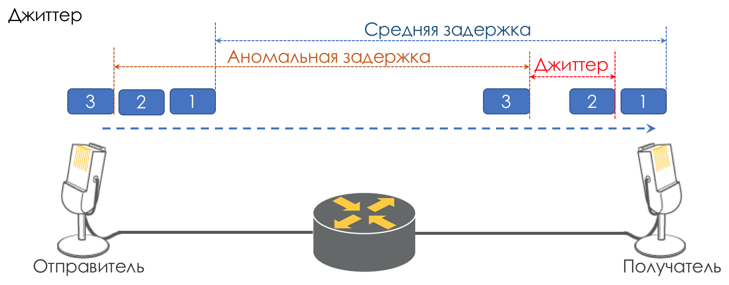
Like latency, jitter is irrelevant for many applications. And even it would seem, what's the difference - the package was delivered, what more?
However, it is important for interactive services.
Take as an example the same telephony. In fact, it is the digitization of analog signals divided into separate chunks of data. The output is a fairly uniform stream of packets. On the receiving side there is a small buffer of a fixed size, in which successively incoming packets are placed. To restore an analog signal, you need a certain number of them. Under conditions of floating delays, the next data chunk may not arrive in time, which is tantamount to loss, and the signal cannot be recovered.
The greatest contribution to the variability of the delay makes just QoS. About this, too, a lot and tedious in the same chapters of the speed limit.
These are the three main characteristics of the quality of the network, but there are two others that also play an important role.
A number of applications such as telephony, NAS , CES are extremely sensitive to unordered packet delivery when they arrive at the recipient in a different order than they were sent. This can lead to loss of connectivity, errors, damage to the file system.
Although unordered delivery is not a formal characteristic of QoS, it definitely refers to network quality.
Even in the case of TCP tolerant to this kind of problems, duplicate ACKs and retransmitts occur.

It is not distinguished as the network quality metric, since in fact its lack results in the three indicated above. However, in our realities, when it should be guaranteed to some applications or, conversely, should be limited under the contract, for example MPLS TE reserves it throughout the entire LSP, it is worth mentioning it, at least as a weak metric.
Speed control mechanisms are discussed in chapters Speed limit.
Why characteristics may deteriorate?
So, we start with a very primitive view that a network device (whether it is a switch, a router, a firewall, or whatever) is just another piece of pipe called a communication channel, the same as a copper wire or an optical cable.

Then all the packages fly through in the same order in which they came and do not experience any additional delays - there is nowhere to linger.
But in fact, each router recovers bits and packets from the signal, does something with them (we do not think about it yet) and then converts the packets back into a signal.
A delay in serialization appears. But in general, it is not scary because it is constant. Not scary as long as the width of the output interface is larger than the input.
For example, at the entrance to the device is a gigabit port, and at the output is a radio relay line 620 MB / s connected to the same gigabit port?
Nobody forbids bullet through a formally gigabit link gigabit traffic.
There is nothing you can do - 380 MB / s will be spilled on the floor.
Here they are - the loss.
But at the same time, I would very much like to see the worst part of it spill out - the video from youtube, and the executive’s telephone conversation with the plant director wasn’t interrupted or even croaked.
I wish the voice had a dedicated line.
Or the input interfaces are five, and the output one, and at the same time, five nodes began to try to infuse traffic to one recipient.
Add a pinch of VoIP theory (an article about which no one has written) - it is very sensitive to delays and their variations.
If for a TCP stream of video from youtube (at the time of writing this article QUIC is still an experiment), even seconds are absolutely free of delays due to buffering, then the director will call the head of the technical department after the first such conversation with Kamchatka.
In older times, when the author of the cycle was still doing lessons in the evenings, the problem was particularly acute. Modem connections had a speed of 56k .
And when such a connection received a one-and-a-half-kilo packet, he occupied the entire line for 200 ms. No one else could pass at that moment. Vote? No, have not heard.
Therefore, the MTU issue is so important - the package should not occupy the interface for too long. The less speedy it is, the less MTU is needed.
These are the delays.
Now the channel is free and the delay is low, in a second someone started downloading a large file and the delays grew. Here it is - jitter.
Thus, it is necessary that voice packets fly through the pipe with minimal delays, and youtube will wait.
Available 620 MB / s should be used for voice, video, and B2B clients buying VPNs. I wish that one traffic did not oppress the other, then you need a band guarantee.
All the above characteristics are universal regarding the nature of the network. However, there are three different approaches to their provision.
No guarantees.
The simplest approach to the implementation of QoS, from which IP networks began and which is practiced to this day - sometimes because it is enough, but more often because no one thought about QoS.
By the way, when you send traffic to the Internet, it will be processed there as BestEffort. Therefore, through VPN, prokinutnye over the Internet (as opposed to VPN provided by the provider), can not very confident to go important traffic, such as a telephone conversation.
In the case of BE, all traffic categories are equal, no preference is given. Accordingly, there is no guarantee for delay / jitter or band.
This approach has a somewhat counterintuitive name - Best Effort, which is misleading the novice with the word “best”.
However, the phrase “I will do my best” means that the speaker will try to do everything that he can, but does not guarantee anything.
Nothing is required to implement BE — this is the default behavior. It is cheap in production, the personnel do not need deep specific knowledge, QoS in this case defies any adjustment.
However, this simplicity and static does not mean that the Best Effort approach is not used anywhere. It finds application in networks with high bandwidth and the absence of congestion and surges.
For example, on transcontinental lines or in networks of some data centers where there is no oversubscription.
In other words, in networks without overloads and where there is no need to treat any traffic in a special way (for example, telephony), BE is quite appropriate.
Provisional reservation of resources for the stream from the source to the recipient.
In the growing unsystematic Internet, the fathers of the MIT, Xerox, ISI networks decided to add an element of predictability, while maintaining its efficiency and flexibility.
So in 1994, the idea of IntServ was born in response to the rapid growth of real-time traffic and the development of multicast. It was reduced then to IS.
The name reflects the desire in the same network to simultaneously provide services for real-time and non-real-time traffic types, providing, first of all, the priority right to use resources through band reservation. The possibility of reusing the band, on which everyone earns, and thanks to what the IP shot, at the same time remained.
The reservation mission was assigned to RSVP, which foreach stream reserves a band on each network device.
Roughly speaking, before setting up a Single Rate Three Color MarkerP session or starting data exchange, end hosts send an RSVP Path indicating the required bandwidth. And if RSVP Resv is back to both of them, they can start communicating. However, if there are no resources available, RSVP returns an error and the hosts cannot communicate or will follow the BE.
Let the bravest of readers now imagine that for any stream on the Internet today a channel will be signaled in advance. Consider that this requires non-zero CPU and memory costs for eachtransit node, postpones the actual interaction for some time, it becomes clear why IntServ was actually a stillborn idea - zero scalability.
In a sense, the modern incarnation of IntServ is MPLS TE with the RSVP version RSVP TE adapted for tag transmission. Although here, of course, not End-to-End and not per-flow.
IntServ is described in RFC 1633 .
The document is in principle curious to evaluate how naive one can be in forecasts.
DiffServ complex.
When it became clear at the end of the 90s that the IntServ IP end-to-end approach failed, the IETF convened in 1997 a working group, Differentiated Services, which developed the following requirements for a new QoS model:
As a result, the epoch-making RFC 2474 ( Definition of the Differentiated Services Field (DS Field) in the IPv4 and IPv6 Headers ) and RFC 2475 ( An Architecture for Differentiated Services ) were born in 1998 .
And then all the way, we will only talk about DiffServ.
What is DiffServ and why does it win against IntServ?
If it is very simple, then the traffic is divided into classes. A package at the entrance to each node is classified and a set of tools is applied to it, which processes packages of different classes differently, thus providing them with a different level of service.
But it just will not .
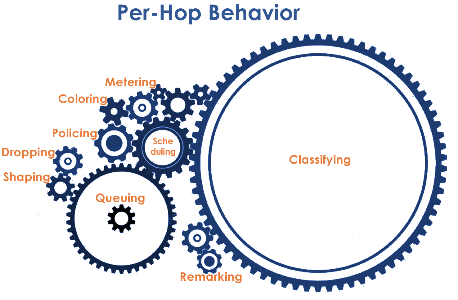
At the heart of DiffServ is the ideological concept of the IP traditionally held in the traditions of PHB - Per-Hop Behavior . Each node on the path of traffic independently makes a decision on how to behave relative to the incoming packet, based on its headers.
The actions of a packet router are called a behavior model ( Behavior). The number of such models is deterministic and limited. Cross-device behaviors in relation to the same traffic may be different, so they are per-hop.
The concepts of Behavior and PHB I will use in the article as synonyms.

The behavior model is determined by the set of tools and their parameters: Policing, Dropping, Queuing, Scheduling, Shaping.
Using existing behaviors, the network can provide various classes of service ( Class of Service ).
That is, different categories of traffic can get a different level of service on the network by applying different PHBs to them.
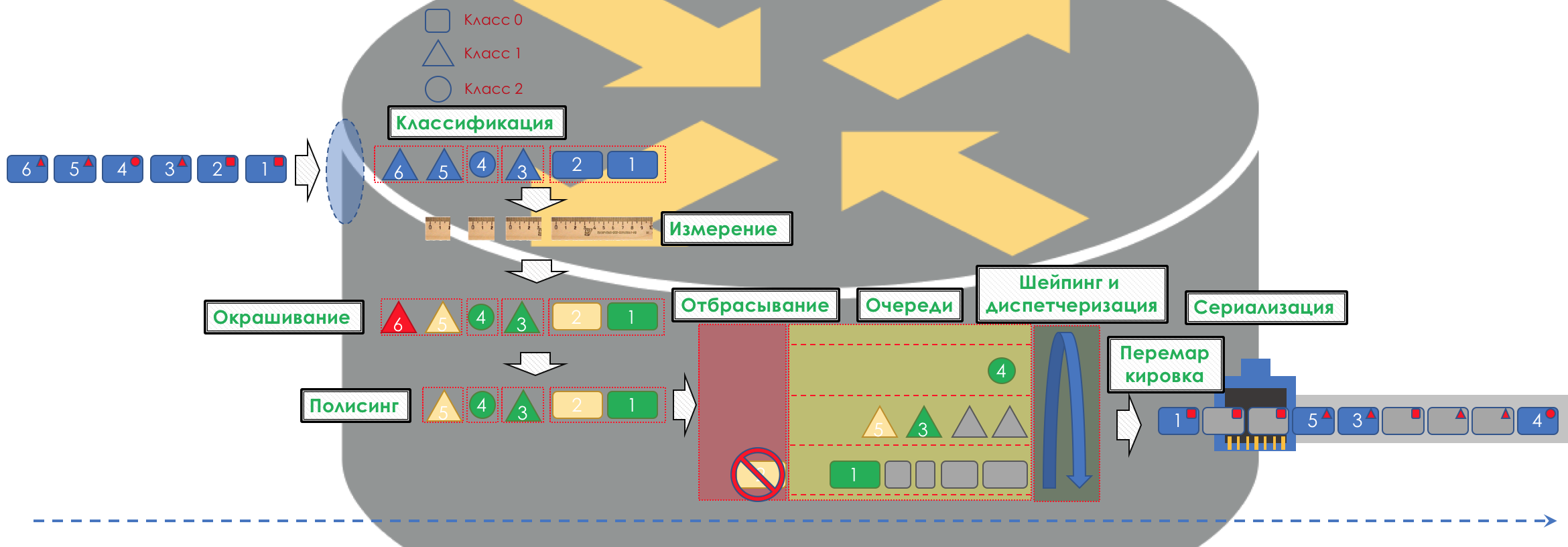
Accordingly, first of all, you need to determine which class of service the traffic belongs to - classification ( Classification ).
Each node independently classifies incoming packets.

After classification, a measurement occurs ( Metering ) - how many bits / bytes of the traffic of a given class has arrived at the router.
Based on the results, the packages can be colored ( Coloring ): green (within the limits of the established limit), yellow (outside the limit), red (all along the coast).
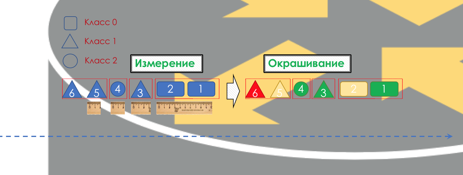
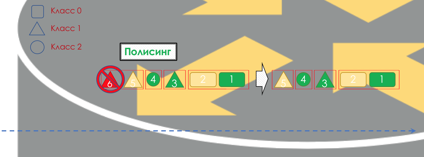
If necessary, further there is policing ( Policing ) (sorry for such a tracing paper, there is a better option - write, I will change). A polisher based on the color of the packet assigns an action to the packet — transfer, discard, or remarry.
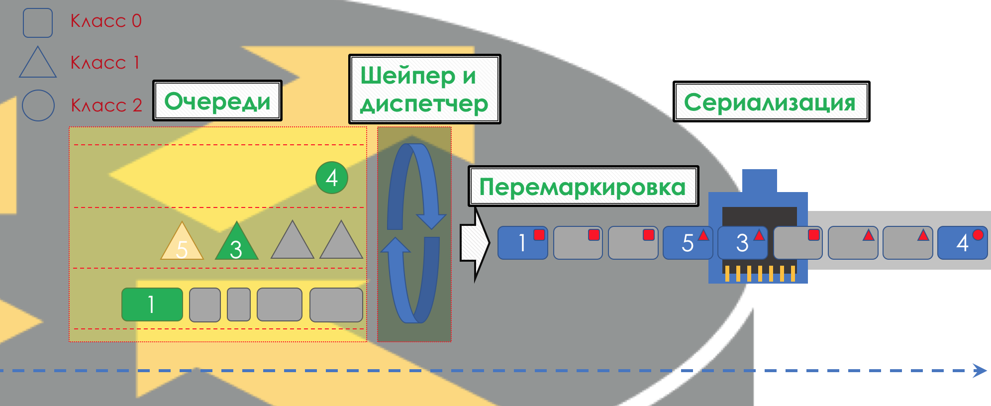
After that, the packet should go into one of the queues ( Queuing ). For each class of service, a separate queue is allocated, which allows them to be differentiated using different PHBs.
But even before the packet enters the queue, it can be dropped ( dropper ) if the queue is full.
If he is green, he will pass, if yellow, then it is likely to be rejected, if the queue is full, and if red - this is a sure suicide bomber. Conventionally, the probability of dropping depends on the color of the packet and the fullness of the queue where it is going to go.
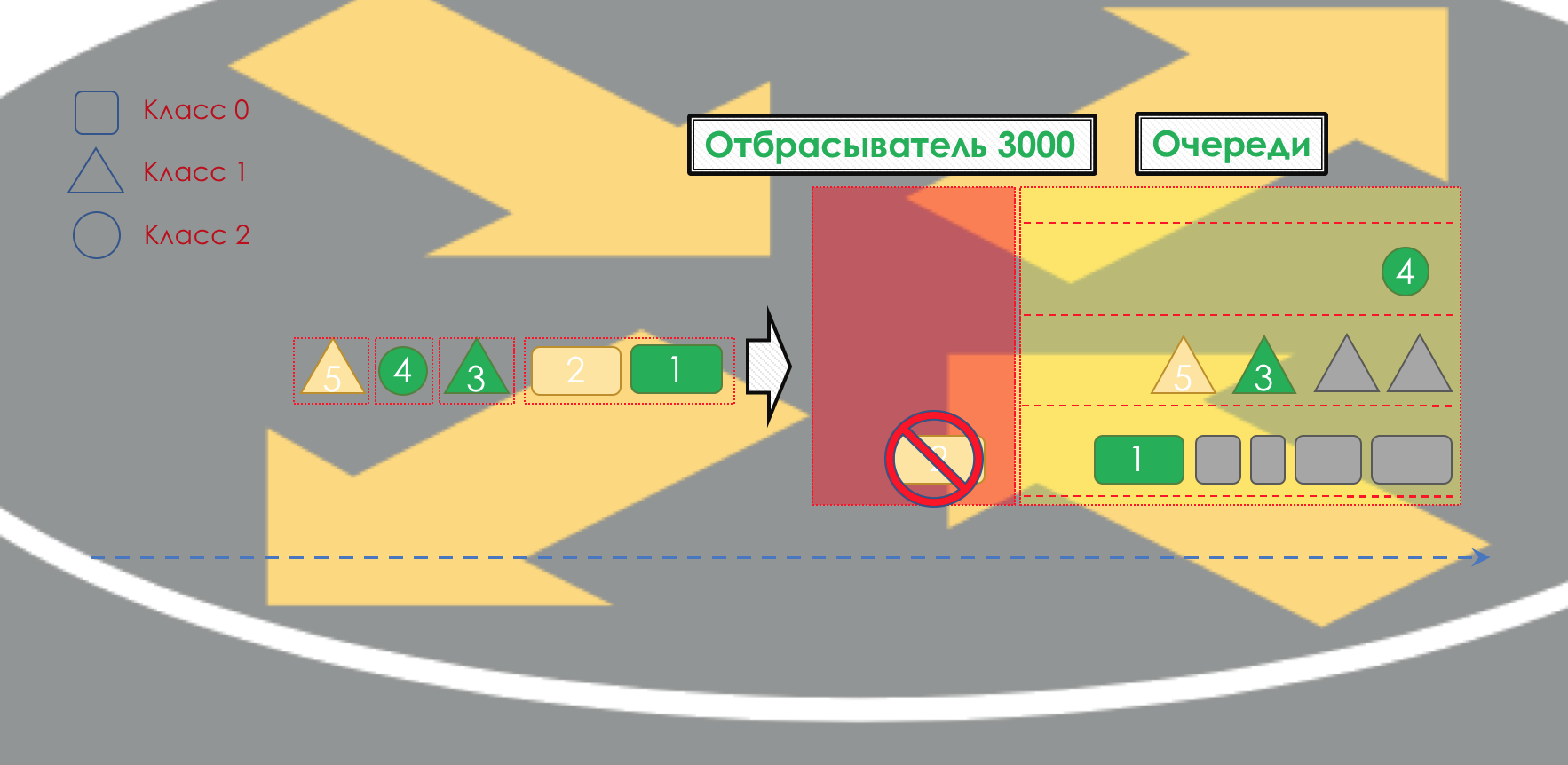
At the exit of the queue, the shaper ( Shaper ), whose task is very similar to the polisher problem, is to limit traffic to the specified value.
You can configure arbitrary shapers for individual queues or even within queues.
On the difference between the shaper and the polisher in the chapter Speed Limit.
All queues should eventually merge into a single output interface.
Remember the situation when on the road 8 lanes merge into 3. Without a traffic controller, this turns into chaos. Separating by queues would not make sense if we had the same output as the output.
Therefore, there is a special dispatcher ( Scheduler ), which cyclically takes out packets from different queues and sends it to the interface ( Scheduling ).
In fact, a bunch of queues and the dispatcher is the most important QoS mechanism that allows you to apply different rules to different traffic classes, one providing a wide band, the other low delays, the third the absence of drops.
Next, the packets already go to the interface, where the packets are converted into a bitstream — serialization ( Serialization ) and then the medium signal.
In DiffServ, the behavior of each node, regardless of the rest, there are no signaling protocols that would report which QoS policy is on the network. At the same time within the network I would like the traffic to be processed in the same way. If only one node will behave differently, the entire QoS policy will go to waste.
For this, firstly, on all routers, the same classes and PHBs are configured for them, and secondly, the packet marking ( Marking ) is used - its belonging to a particular class is written into the header (IP, MPLS, 802.1q).
And the beauty of DiffServ is that the next node can trust this labeling when classifying.
Such a zone of trust, in which the same traffic classification rules and certain behaviors apply, is called the DiffServ domain (DiffServ-Domain ).

Thus, at the entrance to the DiffServ domain, we can classify a packet on the basis of 5-Tuple or interface, mark ( Remark / Rewrite ) it according to the domain rules, and further nodes will trust this marking and not make a complicated classification.
That is, there is no explicit signaling in DiffServ, but a node can tell all of the following which class to provide to this package, expecting it to trust.
At the junctions between DiffServ-domains, you need to coordinate the QoS policy (or not).
The whole picture will look like this:
The threshold for entering the circle of engineers who understand the technology for QoS is much higher than for routing protocols, MPLS, or, forgive me, Radya, STP.
And despite this, DiffServ has earned recognition and implementation on networks around the world, because, as they say, Highly Scaleble.
All further part of the article I will analyze only DiffServ.
Below we will analyze all the tools and processes indicated in the illustration.
In the course of disclosing the topic, I will show some things in practice.
We will work with such a network:
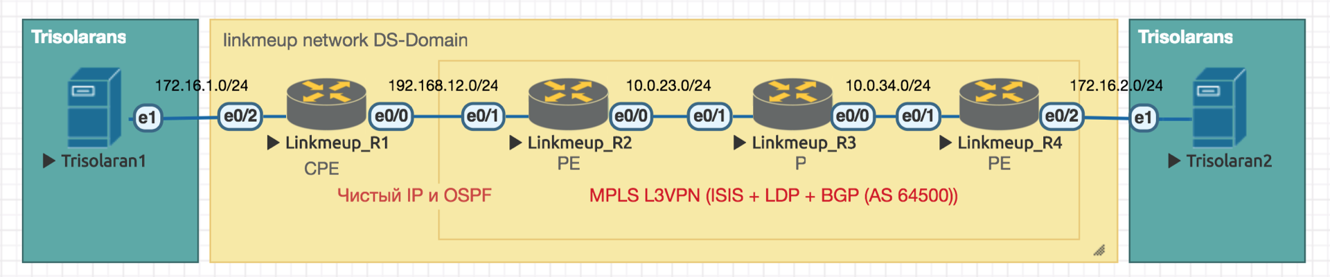
Trisolarans is a client of the linkmeup provider with two connection points.
The yellow area is the DiffServ-domain of the network linkmeup, which has a single QoS policy.
Linkmeup_R1 is a CPE device that is managed by the provider, and therefore in the trusted zone. OSPF is raised with it and the interaction takes place via pure IP.
Within the MPLS + LDP + MP-BGP network core with L3VPN, stretched from Linkmeup_R2 to Linkmeup_R4.
All other comments I will give as needed.
Initial configuration file .
Within its network, the administrator defines the classes of service that he can provide traffic.
Therefore, the first thing that each node does when receiving a packet is its classification.
There are three ways:
The administrator determines the set of service classes that the network can provide and matches them with a numeric value.
We do not trust anyone at the entrance to the DS-domain, so the classification is carried out by the second or third method: the class of service and the corresponding digital value are determined on the basis of addresses, protocols or interfaces.
At the exit of the first node, this digit is encoded in the DSCP field of the IP header (or another field of the Traffic Class: MPLS Traffic Class, IPv6 Traffic Class, Ethernet 802.1p) —remarking occurs.
It is customary to trust this marking inside the DS-domain, therefore transit nodes use the first classification method (BA) - the simplest. No complicated analysis of headings, we look only at the recorded number.
At the junction of the two domains can be classified based on the interface or MF, as I described above, and you can trust the labeling of BA with reservations.
For example, trusting all values except 6 and 7, and 6 and 7 remarking to 5.
Such a situation is possible in the case when the provider connects a legal entity that has its own labeling policy. The provider does not object to keep it, but at the same time does not want traffic to fall into the class in which its network protocol packets are transmitted.
In BA, a very simple classification is used - I see a number - I understand the class.
So what's the number? And what field is it recorded in?
Basically, the classification occurs on a switching header.
I call the switch a header, on the basis of which the device determines where to send the packet so that it becomes closer to the receiver.
That is, if an IP packet arrives at the router, the IP header and the DSCP field are analyzed. If MPLS arrived, MPLS Traffic Class is analyzed.
If an Ethernet + VLAN + MPLS + IP packet arrives on a regular L2 switch, then 802.1p will be analyzed (although this can be changed).
The QoS field accompanies us exactly the same as the IP. The eight-bit TOS field — Type Of Service — was supposed to carry the priority of the packet.
Even before the appearance of DiffServ RFC 791 ( INTERNET PROTOCOL ), the field was described as follows:
IP Precedence (IPP) + DTR + 00.
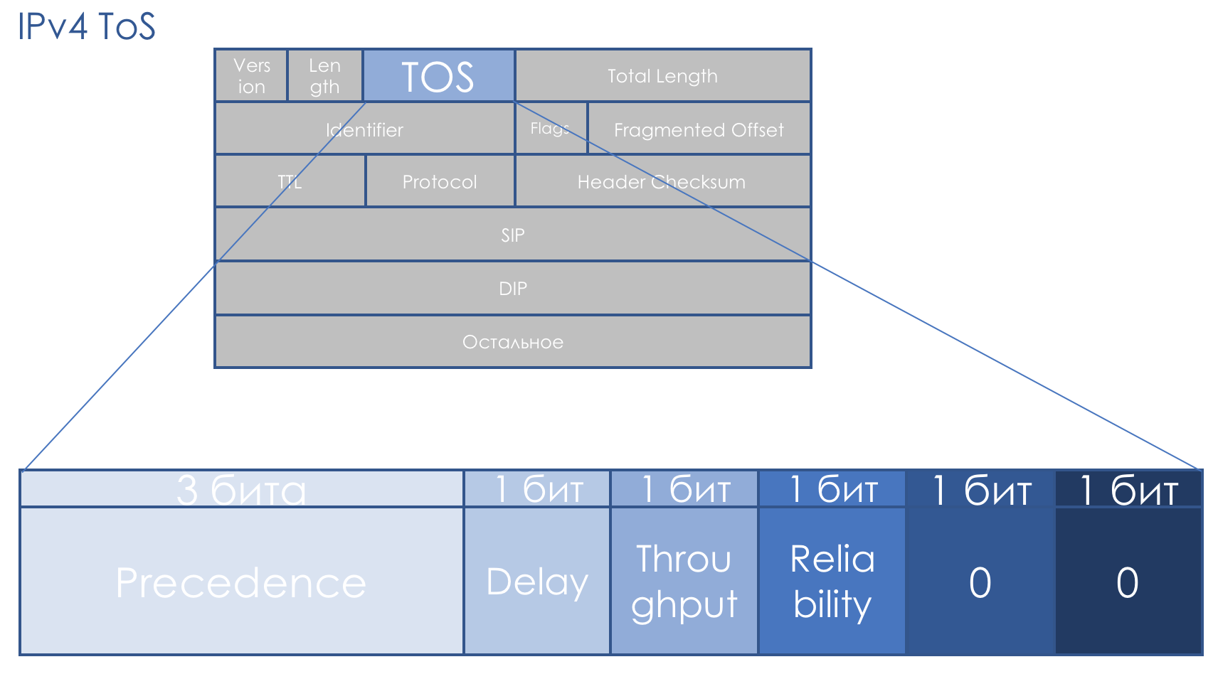
That is, packet priority goes, then the requirements for Delay, Throughput, Reliability (0 - no requirements, 1 - with requirements) .
The last two bits must be zero.
A bit later, in RFC 1349 ( Type of Service in the Internet Protocol Suite ), the TOS field was slightly redefined: The
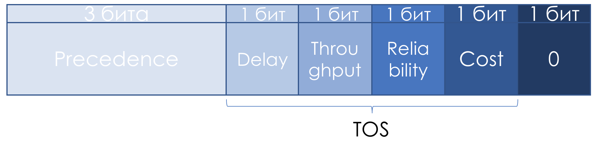
left three bits remained IP Precedence, the next four turned into TOS after adding the Cost bit.
Here's how to read the units in these TOS bits:
Misty descriptions did not contribute to the popularity of this approach.
There was no systematic approach to QoS all the way, there were no clear recommendations on how to use the priority field, the description of the Delay, Throughput and Reliability bits was extremely vague.
Therefore, in the context of DiffServ, the TOS field was again redefined in RFC 2474 ( Definition of Differentiated Services Field (DS Field) in the IPv4 and IPv6 Headers ):
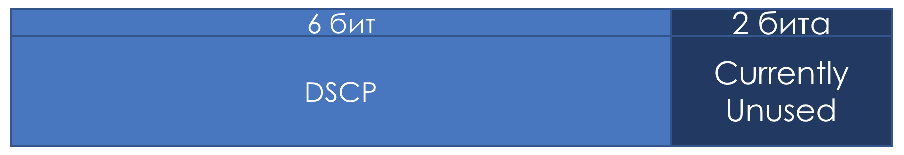
Instead of the IPP and DTRC bits, a six-bit DSCP field was entered - Differentiated Services Code Point , two right bits not Was used.
From this point on, it was the DSCP field that should have become the main DiffServ label: a specific value (code) is written into it, which within a given DS domain characterizes a particular service class required by the packet and its drop priority. This is the same figure.
The administrator can use all 6 bits of DSCP as he pleases, dividing up to a maximum of 64 classes of service.
However, for the sake of compatibility with IP, Precedence for the first three bits retained the role of the Class Selector.
That is, as in IPP, the 3 bits of the Class Selector allow you to define 8 classes.
However, this is no more than an agreement, which, within its DS domain, the administrator can easily ignore and use all 6 bits at will.
Further, I also note that according to the recommendations of the IETF, the higher the value recorded in the CS, the more demanding this traffic to the service.
But this should not be taken as an indisputable truth.
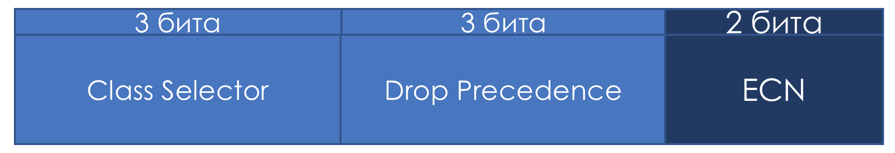
If the first three bits define the traffic class, then the following three are used to indicate the priority of packet drop ( Drop Precedence or Packet Loss Priority (PLP ).
Do not hurt a little practice.
The scheme is the same.
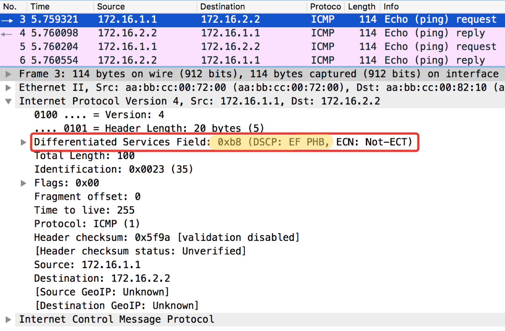
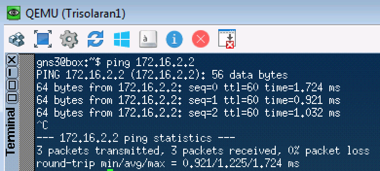
To get started, just send an ICMP request:
Linkmeup_R1. E0 / 0.

pcapng
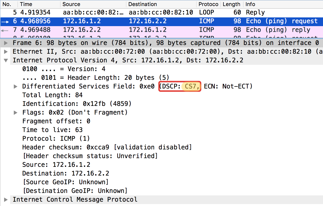
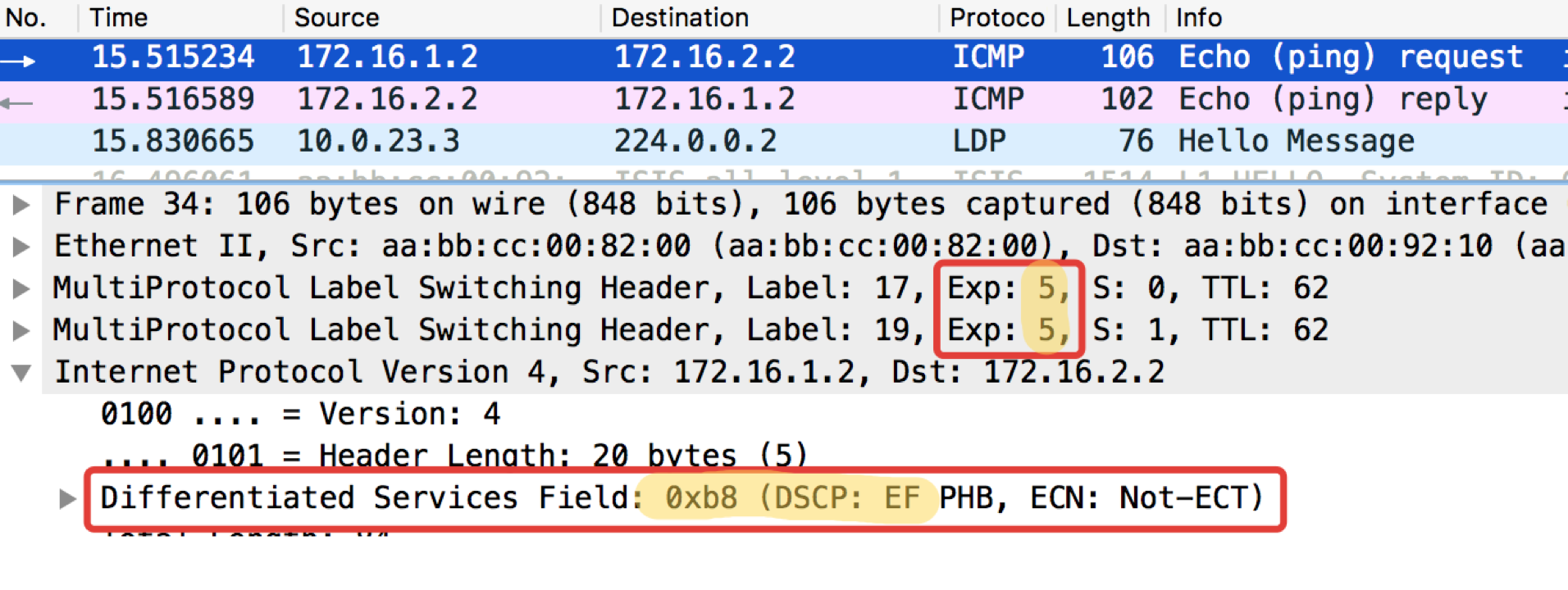
And now with the DSCP value set.
The value 184 is the decimal representation of the binary 10111000. Of these, the first 6 bits are 101110, that is, the decimal 46, and this is the class EF.
Linkmeup_R2. E0 / 0
pcapng
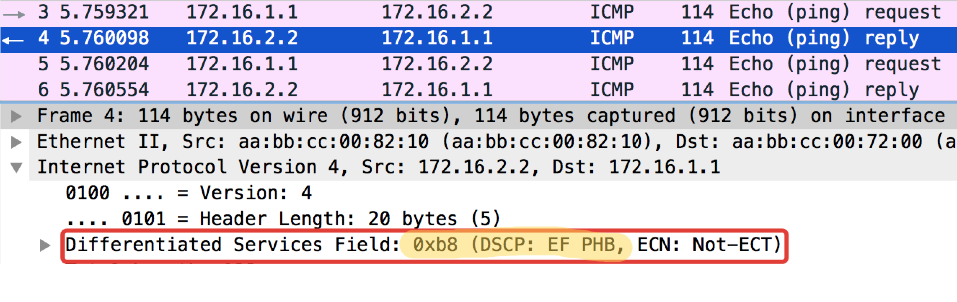
Curious note: the addressee of the pop-ups in ICMP Echo reply sets the same class value as it was in the Echo Request. This is logical - if the sender sent a packet with a certain level of importance, then, obviously, he wants to get it guaranteed back.
Linkmeup_R2. E0 / 0
DSCP classification configuration file.
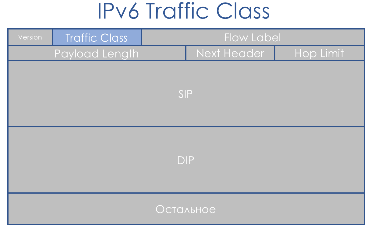
IPv6 is not much different than QoS from IPv4. The eight-bit field, called the Traffic Class, is also split into two parts. The first 6 bits - DSCP - play exactly the same role.
Yes, Flow Label appeared. It is said that it could be used to further differentiate classes. But this idea has nowhere found application in life.
The DiffServ concept was focused on IP networks with IP header routing. That's just bad luck - after 3 years, RFC 3031 ( Multiprotocol Label Switching Architecture ) was published . And MPLS began to seize network providers.
DiffServ was impossible not to spread to him.
By luck, MPLS laid a three-bit EXP field just in case an experimental case. And despite the fact that already long ago in RFC 5462 ( “EXP” Field Renamed to “Traffic Class” Field ) officially became the Traffic Class field, by inertia it is called IExPi.
There is one problem with it - its length is three bits, which limits the number of possible values to 9. It’s not just a little, it’s 3 binary orders of magnitude less than that of DSCP.

Considering that MPLS Traffic Class is often inherited from the DSCP IP packet, we have an archive with loss. Or ... No, you do not want to know ... L-LSP . Uses a combination of Traffic Class + tag value.
Therefore, in terms of service classes, we still have a 1: 1 correspondence, losing only information about Drop Precedence.
In the case of MPLS, the classification, as in IP, can be based on the interface, MF, IP DSCP values or MPLS Traffic Class.
Marking indicates the entry of a value in the Traffic Class field of the MPLS header.
A packet may contain several MPLS headers. For the purposes of DiffServ, only the top one is used.
There are three different remarking scenarios when moving a packet from one pure IP segment to another via an MPLS domain: (this is just an excerpt from the article ).
The scheme is the same:
The configuration file is the same.
The linkmeup network map has a transition from IP to MPLS on Linkmeup_R2.
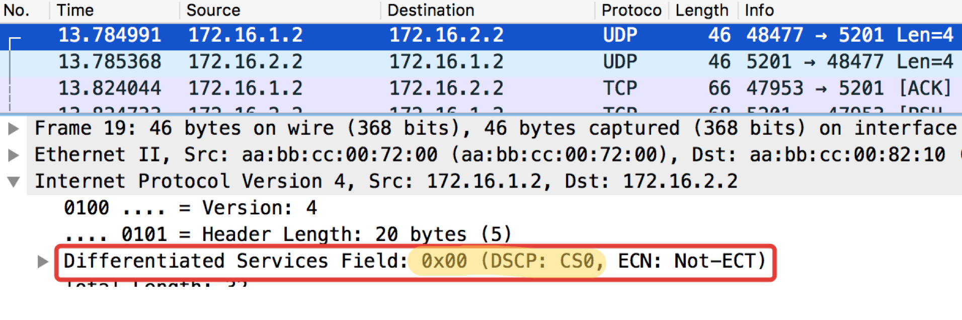
Let's see what happens with the marking when pinging ip 172.16.2.2 source 172.16.1.1 tos 184 .
Linkmeup_R2. E0 / 0.

pcapng
So, we see that the original EF tag in IP DSCP has been transformed into a value of 5 of the EXP MPLS field (it’s the Traffic Class, remember this) of both the VPN header and the transport one.
Here we are witnessing the Uniform mode of operation.
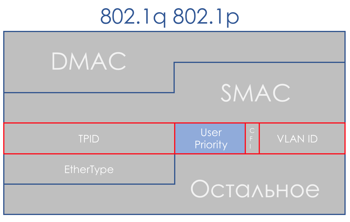
The absence of a priority field in 802.3 (Ethernet) is explained by the fact that Ethernet was originally planned solely as a solution for the LAN segment. For modest money, you can get excess bandwidth, and the bottleneck will always be uplink - there is nothing to worry about prioritizing.
However, it soon became clear that the financial attractiveness of Ethernet + IP brings this bundle to the level of the backbone and the WAN. Yes, and cohabitation in one LAN-segment of torrents and telephony needs to be resolved.
Fortunately, by this time, 802.1q (VLAN) arrived, in which a 3-bit (again) field was allocated to priorities.
In terms of DiffServ, this field allows you to define the same 8 traffic classes.
When receiving a packet, the network device of the DS-domain in most cases takes into consideration the header it uses for switching:
Although this behavior can be changed: Interface-Based and Multi-Field classification. And you can sometimes even explicitly say in the CoS field of which title to look.
This is the easiest way to classify packages in the forehead. Everything that has been poured into the specified interface is marked with a specific class.
In some cases, this granularity is enough, so Interface-based is used in life.
The scheme is the same:
Setting up QoS policies in the equipment of most vendors is divided into stages.
We start the usual ping on 172.16.2.2 (Trisolaran2) with Trisolaran1:
And in the dump between Linkmeup_R1 and Linkmeup_R2 we will see the following:
pcapng
Interface-Based classification configuration file.
The most common type of classification at the entrance to the DS-domain. We do not trust the existing marking, but on the basis of the packet headers we assign a class.
This is often a way to “turn on” QoS altogether, in the case where senders do not affix a label.
A rather flexible tool, but at the same time cumbersome - you need to create difficult rules for each class. Therefore, inside the DS-domain is more relevant BA.
The scheme is the same:
From the practical examples above, it is clear that network devices by default trust labeling of incoming packets.
This is fine inside the DS domain, but unacceptable at the entry point.
And now let's not blindly trust? On Linkmeup_R2 ICMP we will mark as EF (for example only), TCP as AF12, and everything else CS0.
This will be the MF (Multi-Field) classification.
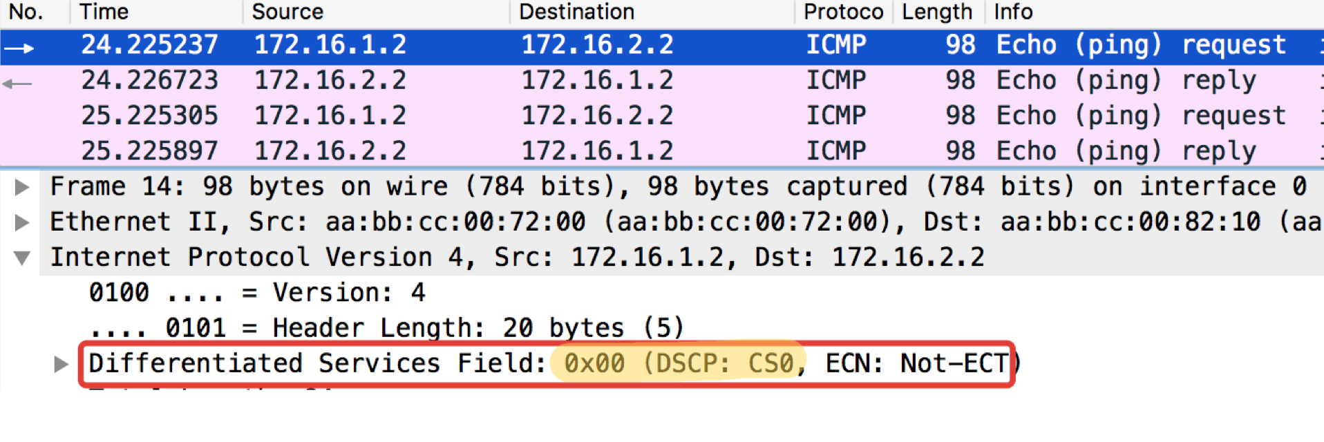
ICMP test from the final host Trisolaran1. In no way do we deliberately indicate the class — the default is 0.
I have already removed the policy with Linkmeup_R1, so traffic comes in as CS0, not CS7.

Here are two dumps alongside, with Linkmeup_R1 and Linkmeup_R2:
Linkmeup_R1. E0 / 0.
pcapng
Linkmeup_R2. E0 / 0.
pcapng
It can be seen that after the classifiers and remarking on Linkmeup_R2 on ICMP packets, not only the DSCP was changed to EF, but the MPLS Traffic Class became equal to 5.
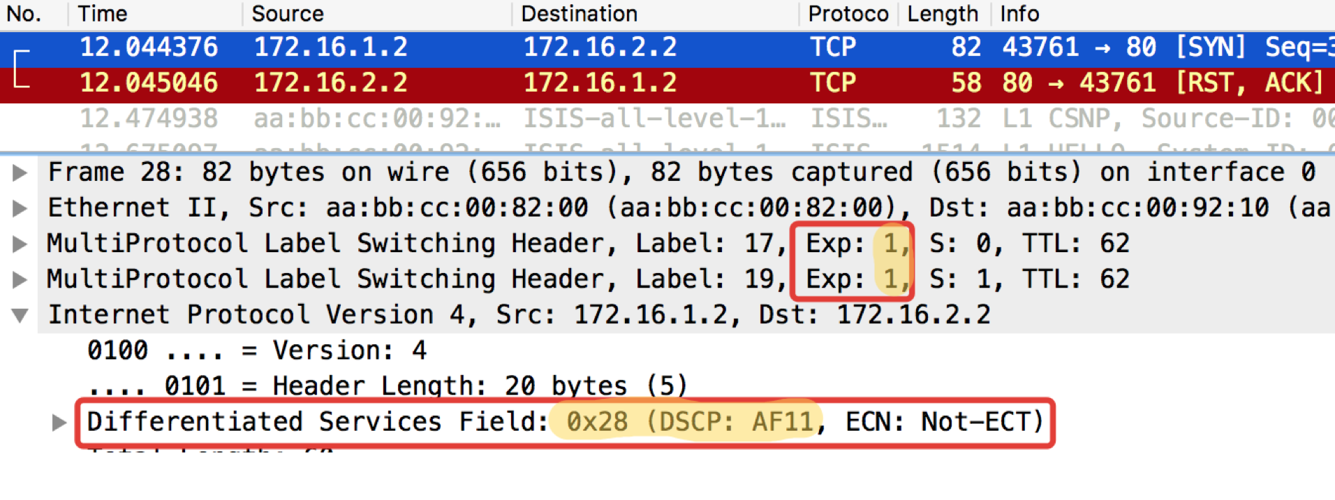
A similar test with telnet 172.16.2.2. 80 - so check TCP:
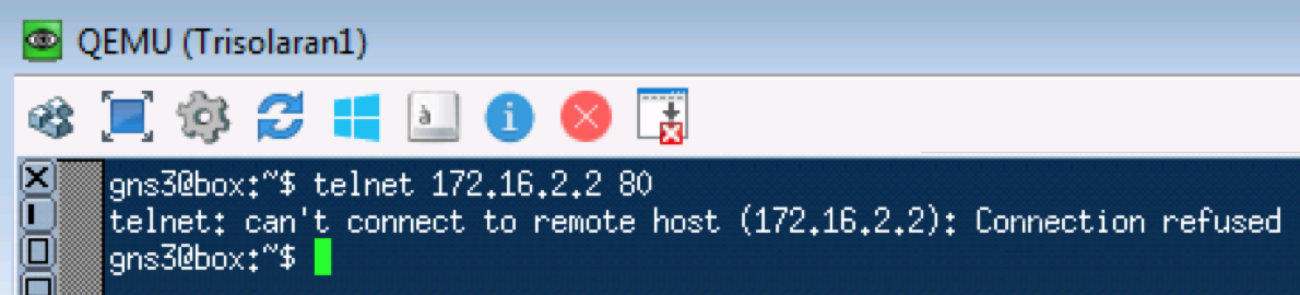
Linkmeup_R1. E0 / 0.

pcapng
Linkmeup_R2. E0 / 0.
pcapng
CHITO - What And Required to Expect. TCP is transmitted as AF11.
The next test will check for UDP, which should go to CS0 according to our classifiers. To do this, use iperf (bring it to Linux Tiny Core via Apps). On the remote side iperf3 -s - we start the server, on the local iperf3 -c -u -t1 - the client ( -c ), the UDP protocol ( -u ), test for 1 second ( -t1 ).
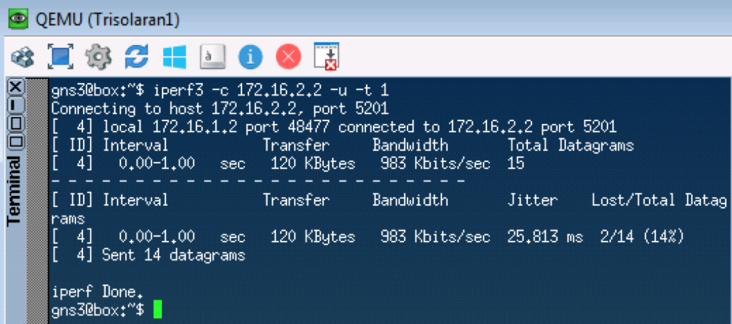
Linkmeup_R1. E0 / 0.
pcapng
Linkmeup_R2. E0 / 0

pcapng
From this point on, everything that comes into this interface will be classified according to the configured rules.
Once again: at the entrance to the DS-domain classification MF, Interface-based or BA can occur.
Between the DS-domain nodes, the packet in the header carries a sign about the class of service it needs and is classified by BA.
Regardless of the method of classification after it, the package is assigned an internal class within the device, according to which it is processed. The header is removed at the same time, and the bare (no) package travels to the exit.
And on output, the inner class is converted to the CoS field of the new header.
That is, Title 1 ⇒ Classification ⇒ Internal Service Class ⇒ Title 2.
In some cases, you need to display the header field of one protocol in the header field of another, for example, the DSCP in the Traffic Class.
This happens just through the intermediate internal marking.
For example, DSCP Header ⇒ Classification ⇒ Internal Service Class ⇒ Traffic Class Header.
Formally, inner classes can be called arbitrarily or simply numbered, and they only correspond to a specific queue.
At the depth to which we are immersed in this article, it doesn’t matter what they are called, it’s important that a specific behavior model is put into correspondence with specific values of the QoS fields.
If we are talking about specific QoS implementations, then the number of service classes that a device can provide is no more than the number of available queues. Often, there are eight of them (either under the influence of the IPP or under the unwritten agreement). However, depending on the vendor, device, board, there may be more or less.
That is, if there are 4 queues, then the service classes simply do not make sense to do more than four.
We'll talk about this in more detail in the hardware chapter.
In terms of PHB, there is absolutely no difference what is used for classification - DSCP, Traffic Class, 802.1p.
Inside the device, they become traffic classes defined by the network administrator.
That is, all these markings are a way to tell the neighbors what class of service they should assign to this package. This is about how the BGP Community, which do not mean anything by themselves, until the policy of their interpretation is defined on the network.
Standards do not standardize at all exactly which classes of service should exist, how to classify and label them, and which PHB to apply to them.
It is at the mercy of vendors and network administrators.
We have only 3 bits - we use as we want.
It's good:
This is bad:
Therefore, the IETF in 2006 released a training manual on how to approach the differentiation of services: RFC 4594 ( Configuration Guidelines for DiffServ Service Classes ).
Further briefly the essence of this RFC.
DF - Default Forwarding
Standard forwarding.
If the behavior class is not specifically assigned a behavior model, it will be processed exactly by Default Forwarding.
This is the Best Effort - the device will do everything possible, but does not guarantee anything. Dropping, reordering, unpredictable delays and floating jitter are possible, but this is not accurate.
This model is suitable for undemanding applications, such as mail or file uploads.
There is, by the way, PHB and even less certain - A Lower Effort .
AF - Assured Forwarding
Guaranteed Shipment.
This is an improved BE. Here are some guarantees, such as strips. Drops and floating delays are still possible, but to a much lesser extent.
The model is suitable for multimedia: Streaming, video conferencing, online games.
RFC 2597 ( Assured Forwarding PHB Group ).
EF - Expedited Forwarding
Emergency Shipping.
All resources and priorities are thrown here. This is a model for applications that need no loss, short delays, stable jitter, but they are not greedy for the band. Like, for example, telephony or wire emulation service (CES - Circuit Emulation Service).
Losses, disordering, and floating delays in EF are extremely unlikely.
RFC 3246 ( An Expedited Forwarding PHB ).
CS - Class Selector
These are behaviors designed to maintain backward compatibility with IP Precedence on networks that can do DS.
The following classes exist in IPP: CS0, CS1, CS2, CS3, CS4, CS5, CS6, CS7.
There is not always a separate PHB for all of them, usually two or three of them, and the rest are simply translated into the nearest DSCP class and receive the corresponding PHB.
For example, a packet labeled CS 011000 can be classified as 011010.
Of the CS, only CS6, CS7, which are recommended for the NCP - Network Control Protocol and require a separate PHB, are preserved in the equipment.
Like EF, PHB CS6,7 are designed for those classes that have very high requirements for delays and losses, but to some extent tolerant of discrimination in the band.
The PHB challenge for CS6.7 is to provide a level of service that eliminates drops and delays even in the event of an extreme overload of the interface, chip, and queues.
It is important to understand that PHB is an abstract concept - and in fact they are realized through mechanisms available on real equipment.
Thus, the same PHB defined in the DS domain may differ on Juniper and Huawei.
Moreover, a single PHB is not a static set of actions, PHB AF, for example, can consist of several options that differ in the level of guarantees (band, permissible delays).
The IETF took care of the administrators and defined the main categories of applications and the aggregating classes of services.
I will not be wordy here, just insert a couple of tablets from this Guideline RFC.
Application categories:

Requirements for network characteristics:
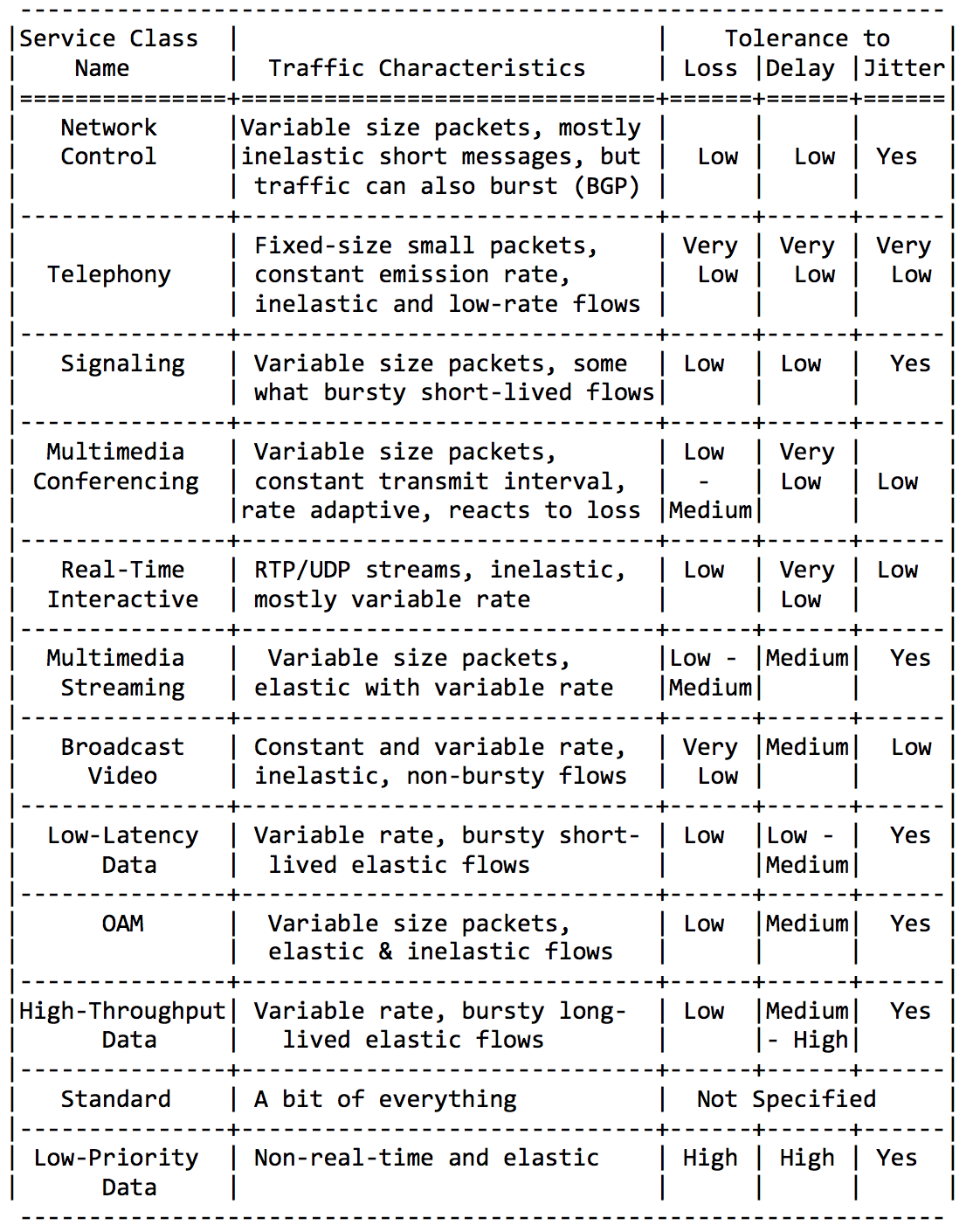
Finally, recommended class names and corresponding DSCP values:

By combining the above classes in different ways (to fit the 8 available ones), you can get QoS solutions for different networks.
The most frequent is, perhaps, the following: An

absolutely undemanding traffic is marked with a DF (or BE) class - it receives attention according to the residual principle.
PHB AF serves classes AF1, AF2, AF3, AF4. They all need to provide a strip, to the detriment of delays and losses. Losses are controlled by the Drop Precedence bits, so they are called AFxy, where x is the class of service, and y is Drop Precedence.
EF needs some kind of minimum bandwidth guarantee, but more importantly, guaranteeing delays, jitter and no loss.
CS6, CS7 require even less bandwidth, because it is a trick of service packets, in which bursts are still possible (BGP Update, for example), but losses and delays are unacceptable in it - what is the use of BFD with a timer of 10 ms if Hello is dried in queues of 100 ms?
That is, 4 classes out of 8 available given under AF.
And despite the fact that in fact they usually do this, I repeat that these are only recommendations, and nothing in your DS domain prevents you from assigning three classes EF and only two classes - AF.
At the node entry, a packet is classified based on the interface, MF, or its labeling (BA).
Marking is the value of the DSCP fields in IPv4, the Traffic Class in IPv6 and in MPLS or 802.1p in 802.1q.
There are 8 classes of service that aggregate various categories of traffic. Each class is assigned its own PHB, which meets the requirements of the class.
According to the IETF recommendations, the following classes of services are distinguished, these are CS1, CS0, AF11, AF12, AF13, AF21, CS2, AF22, AF23, CS3, AF31, AF32, AF33, CS4, AF41, AF42, AF43, CS5, EF, CS6, CS7 in order of increasing traffic importance.
Of these, you can choose a combination of 8 that can actually be encoded in the CoS fields.
The most common combination: CS0, AF1, AF2, AF3, AF4, EF, CS6, CS7 with 3 color gradations for AF.
Each class is assigned a PHB, of which there are 3 - Default Forwarding, Assured Forwarding, Expedited Forwarding in order of increasing severity. A little apart is the PHB Class Selector. Each PHB can vary the parameters of the instruments, but more on that later.
In an unloaded network, QoS is not needed, they said. Any QoS issues are resolved by link extensions, they said. With Ethernet and DWDM, we are never threatened with overloading the lines, they said.
They are the ones who do not understand what QoS is.
But reality beats VPNs on RKN.
There are actually only three groups of QoS provisioning tools that actively handle packages:
But all of them would be largely useless if not for the queue.
In the amusement park you can not give someone priority, if you do not organize a separate queue for those who paid more.
The same situation in the networks.
If all traffic is in the same queue, you will not be able to pull important packets out of its middle to give them priority.
That is why, after classification, packages are placed in the appropriate queue of this class.
And then one queue (with voice data) will move quickly, but with a limited band, the other will be slower (streaming), but with a wide band, and some resources will fall on the residual principle.
But within the limits of each separate turn the same rule operates - it is impossible to pull out a package from the middle - only from its headboard.
Each queue has a certain limited length. On the one hand, this is dictated by hardware limitations, and on the other hand, it makes no sense to keep packets in the queue for too long. VoIP packet is not needed if it is delayed for 200ms. TCP will request a re-send, conditionally, after the expiration of the RTT (configured in sysctl). Therefore, dropping is not always bad.
Developers and designers of network equipment have to find a compromise between attempts to save the package as long as possible and, on the contrary, to prevent the waste of bandwidth, trying to deliver the package that no one else needs.
In a normal situation, when the interface / chip is not overloaded, the buffer utilization is near zero. They absorb short-term bursts, but this does not cause them to be filled for a long time.
If more traffic arrives than the switching chip or output interface can handle, the queues begin to fill up. And chronic utilization is higher than 20-30% - this is already a situation to which measures need to be taken.
In the life of any router there comes a time when the queue is full. Where to put the package, if you put it absolutely nowhere - all, the buffer is over, absolutely, and will not be, even if you search well, even if you pay extra.
There are two ways here: discard either this package or those that have already been scored.
If those that are already in the queue, then consider that it is gone.
And if this, then consider that he did not come.
These two approaches are called Tail Drop and Head Drop .
Tail Drop - the easiest queue management mechanism - discard all newly arrived packets that do not fit in the buffer.

Head Drop discards packets that have been in line for a very long time. It is better to throw them away than to try to save them, because they are most likely useless. But more actual packages that came to the end of the queue will have more chances to arrive on time. Plus, Head Drop will allow you not to load the network with unnecessary packages. Naturally, the oldest packages are those in the head queue, hence the name of the approach.

Head Drop has another unobvious advantage - if the packet is dropped at the beginning of the queue, the recipient will soon find out about the overload on the network and inform the sender. In the case of Tail Drop, the information about the dropped packet will reach, perhaps hundreds of milliseconds later - while it comes from the tail of the queue to its head.
Both mechanisms work with differentiation by queues. That is, in fact, it is not necessary for the entire buffer to overflow. If the 2nd stage is empty, and zero to the outset, then I will only drop packets from zero.

Tail Drop and Head Drop can work simultaneously.
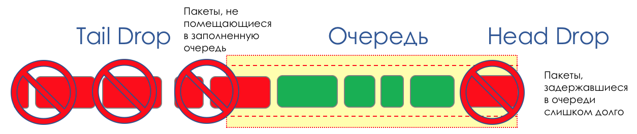
Tail and Head Drop is a forehead congestion avoidance. I can even say - this is his absence.
Do nothing until the queue is 100% full. And after that, all new arrivals (or long-delayed) packets begin to be discarded.
If to achieve the goal you do not need to do anything, then somewhere there is a nuance.
And this nuance is TCP.
Let us recall ( deeper and extremely deep ) how TCP works - speech about modern implementations.
There is a Sliding Window (Sliding Window or rwnd - Reciever's Advertised Window ), which is controlled by the recipient, telling the sender how much you can send.
And there is an overload window ( CWND - Congestion Window), which responds to network problems and is controlled by the sender.
The data transfer process begins with a slow start ( Slow Start ) with an exponential growth of CWND. With each confirmed segment, 1 MSS size is added to CWND, that is, it actually doubles in a time equal to RTT (data goes there, back ACK) (Reno / NewReno speech).
For example,

Exponential growth continues to a value called ssthreshold (Slow Start Threshold), which is specified in the TCP configuration on the host.
Next begins lineargrowth of 1 / CWND for each confirmed segment until either it stops at RWND or losses start (loss of evidence is repeated confirmation (Duplicated ACK) or lack of confirmation at all).
As soon as a segment loss is detected, TCP Backoff occurs - TCP dramatically reduces the window, actually reducing the sending speed, - and the Fast Recovery mechanism starts :
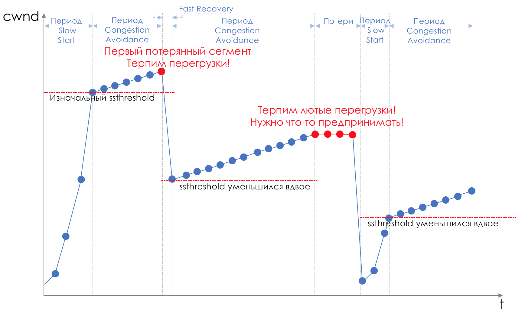
Loss can mean either a complete collapse of some network segment and then consider that it has disappeared, or overload on the line (read buffer overflow and discard segment of this session).
This is TCP's method of maximizing the utilization of available bandwidth and overloading. And it is quite effective.
But what does Tail Drop lead to?
Learn more about changes in TCP mechanisms in RFC 2001 ( TCP Slow Start, Congestion Avoidance, Fast Retransmit, and Fast Recovery Algorithms ).
This is a typical illustration of a situation called global TCP global synchronization ( Global TCP Synchronization ):

Global - because many sessions established through this node suffer.
Synchronization , because they suffer at the same time. And the situation will be repeated as long as there is an overload.
TCP - because UDP, which does not have congestion control mechanisms, is not affected by it.
There would be nothing bad in this situation if it did not cause the suboptimal use of the strip - the gaps between the teeth of the saw are money spent in vain.
The second problem is TCP Starvation - TCP depletion. While TCP slows down its speed to reduce the load (we will not be cunning - first of all, in order to transfer its data for sure), UDP sends all of its moral suffering over the datagram — it sends as much as it can.
So, the amount of TCP traffic is decreasing, and UDP is growing (possibly), the next cycle is Loss - Fast Recovery happens on a lower threshold. UDP takes up the free space. Total TCP traffic drops.
How to solve a problem, it is better to avoid it. Let's try to reduce the load before it fills the queue, using Fast Recovery / Slow Start, which has just been against us.
And what if we take the drops to smear over some part of the buffer?
Relatively speaking, to start dropping random packets when the queue is 80% full, forcing some TCP sessions to reduce the window and, accordingly, speed.
And if the queue is 90% full, we begin to randomly discard 50% of the packets.
90% - the probability increases up to Tail Drop (100% of new packets are discarded).
The mechanisms that implement such queue management are called AQM - Adaptive (or Active) Queue Management
This is exactly how RED works .
Early Detection - we fix potential overload;
Random - discard packets in random order.
Sometimes RED is decrypted (in my opinion semantically more correctly), as a Random Early Discard.
Graphically, it looks like this:
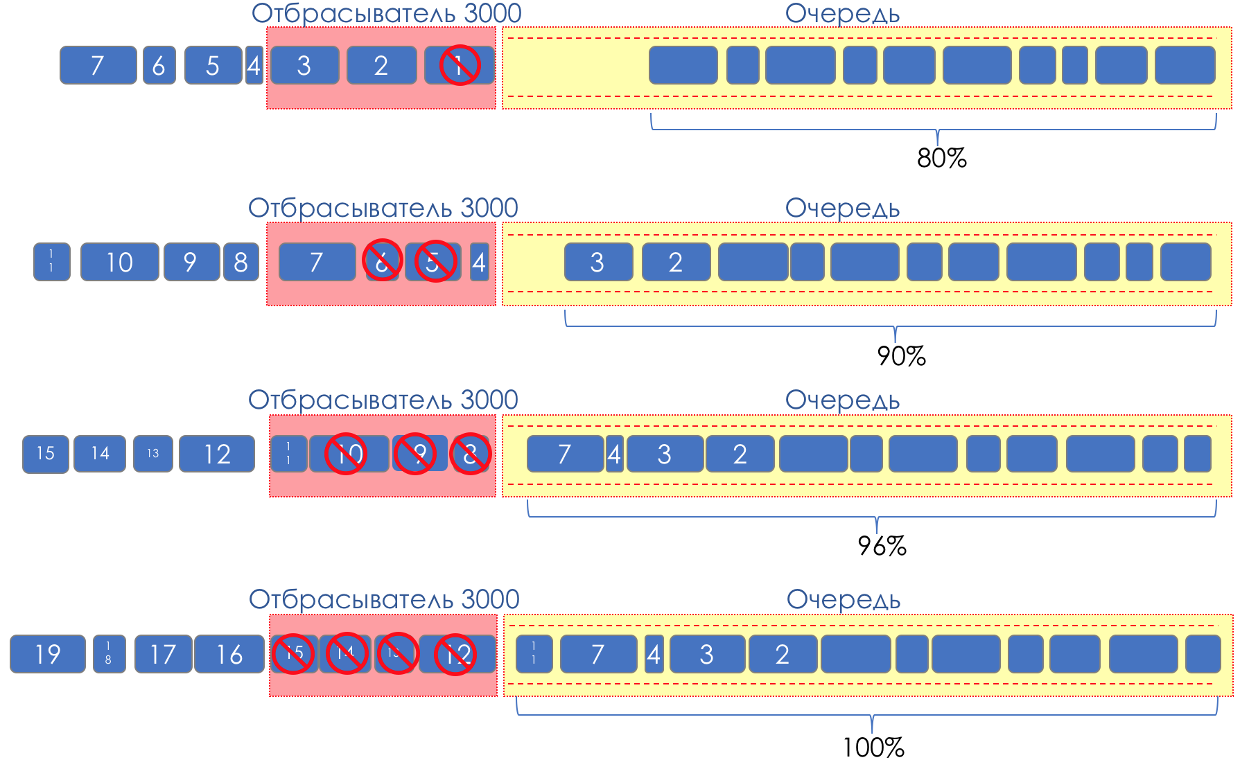
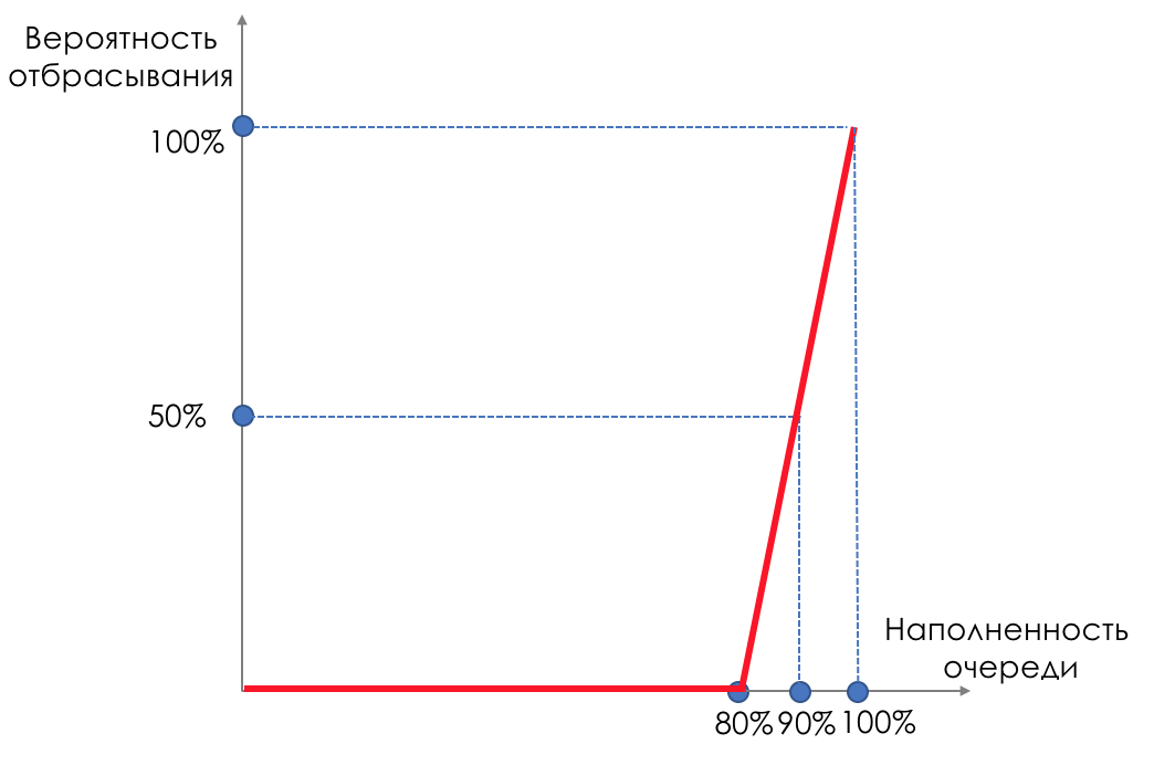
Before filling the buffer, 80% of the packets are not discarded at all - the probability is 0%.
From 80 to 100 packets begin to be discarded, and the more, the higher the filling of the queue.
So the percentage grows from 0 to 30.
A side effect of RED is that aggressive TCP sessions will rather slow down, simply because their packets are many and they are more likely to be dropped.
The inefficiency of using the strip RED decides that it dulls a much smaller part of the sessions without causing such a serious drawdown between the teeth.
Exactly for the same reason, UDP cannot occupy everything.
But at the hearing of all, probably, still WRED . The astute reader linkmeup has already suggested that this is the same RED, but weighted by queues. And he was not quite right.
RED operates within the same queue. It makes no sense to look back at EF if BE is overflowed. Accordingly, weighing by queues will not bring anything.
This is where Drop Precedence works.
And within the same queue, packets with different priority drops will have different curves. The lower the priority, the more likely it is to slam it.

There are three curves:
Red - less priority traffic (in terms of dropping), yellow - more, green - maximum.
Red traffic begins to be discarded when the buffer is full by 20%, from 20 to 40 it drops to 20%, then - Tail Drop.
Yellow starts later - from 30 to 50, it is discarded up to 10%, then - Tail Drop.
Green is the least susceptible: from 50 to 100 it grows smoothly to 5%. Next - Tail Drop.
In the case of DSCP, this could be AF11, AF12 and AF13, respectively green, yellow and red.

Very important here is that it works with TCP and it is absolutely not applicable to UDP.
Either the application using UDP ignores the loss, as in the case of telephony or streaming video, and this adversely affects what the user sees.
Either the application itself controls the delivery and asks to resend the same package. However, it is not at all obliged to ask the source to reduce the transmission rate. And instead of reducing the load, an increase due to retransmit is obtained.
That is why only Tail Drop is used for EF.
For CS6, CS7 also uses Tail Drop, since there are no high speeds expected there and WRED will not solve anything.
For AF, apply WRED. AFxy, where x is the service class, that is, the queue to which it falls, and y is the drop priority — that same color.
For BE, the decision is made based on the traffic prevailing in this queue.
Within the same router, special internal packet marking is used that is different from the one that the headers carry. Therefore, MPLS and 802.1q, where it is not possible to encode Drop Precedence, can be processed in queues with different drop priorities.
For example, the MPLS packet arrived at the node, it does not carry the Drop Precedence marking, however, by the results of the polysing it turned yellow and could be discarded before being placed in a queue (which may be determined by the Traffic Class field).
It should be remembered that the whole rainbow exists only inside the node. There is no color concept in the line between neighbors.
Although it is possible to encode the color in the Drop Precedence part of the DSCP.
Well, what to do when it became bad after all?
When everything is bad, priority should be given to more important traffic. The importance of each package is determined at the classification stage.
But what is bad?
Optionally, all buffers must be clogged for applications to begin to experience problems.
The simplest example is voice packs that crowd over large packs of large application packs that download a file.
This will increase latency, ruin jitter and possibly cause drops.
That is, we have problems with providing quality services in the absence of actual overloads.
This problem is designed to solve the mechanism of congestion management (Congestion Management).
The traffic of different applications is divided into queues, as we have already seen above.
That's just as a result, everything should merge into one interface again. Serialization still happens sequentially.
How do different queues manage to provide different levels of services?
Differently withdraw packets from different queues.
Engaged in this dispatcher.
We will look at most of the existing dispatchers today, starting with the simplest:
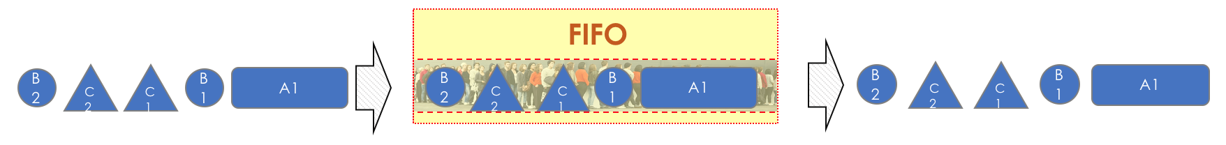
The simplest case, essentially the absence of QoS, is that all traffic is treated the same way - in one queue.
Packages leave the queue exactly in the order in which they got there, hence the name: first entered - first and out .
FIFO is neither a dispatcher in the full sense of the word, nor is it a DiffServ mechanism at all, because in no way does it share classes.
If the queue starts to fill up, delays and jitter start to grow, you cannot control them, because you cannot pull an important packet from the middle of the queue.
Aggressive TCP sessions with a packet size of 1500 bytes can occupy the entire queue, causing small voice packets to suffer.
In FIFO, all classes are merged into CS0.
However, despite all these shortcomings, this is how the Internet works now.
Most FIFO vendors still have a default dispatcher with one queue for all transit traffic and another for locally generated service packets.
It is simple, it is extremely cheap. If the channels are wide and the traffic is low, everything is fine.
The quintessence of the idea that QoS - for the poor - expand the band, and customers will be satisfied, and your salary will grow multiply.
This is the only time when network equipment worked.
But very soon, the world is faced with the fact that it just will not work.
With the trend towards convergent networks, it became clear that different types of traffic (service, voice, multimedia, Internet surfing, file sharing) are fundamentally different network requirements.
FIFO was not enough, so we created several queues and began to produce traffic control schemes.
However, a FIFO never leaves our lives: within each of the queues, packets are always processed according to the FIFO principle.
The second most complex mechanism and an attempt to divide the service into classes is a priority queue .
Traffic is now decomposed into several queues according to its class — priority (for example, although not necessarily the same BE, AF1-4, EF, CS6-7). The dispatcher enumerates one queue after another.
First, it skips all packets from the highest priority queue, then from less, then from less. And so in a circle.
The dispatcher does not begin to withdraw low priority packets until the high priority queue is empty.

If at the moment of processing of low-priority packets a packet arrives in a higher priority queue, the dispatcher switches to it and only after emptying it returns to the others.
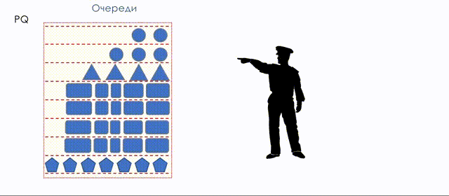
PQ works almost as much in the forehead as a FIFO.
It is great for such types of traffic as protocol packets and voice, where delays are critical, and the total volume is not very large.
Well, you see, it is not necessary to hold BFD Hello due to the fact that several large video chunks came from YouTube?
But here lies the lack of PQ - if the priority queue is loaded with traffic, the dispatcher will never switch to others at all.
And if some Doctor Evil, in search of methods to conquer the world, decides to mark all of his villainous traffic with the highest black mark, all the others will humbly wait and then be discarded.
There is no need to talk about a guaranteed lane for each queue either.
High-priority queues can be cut to the speed of the traffic processed in them. Then others will not starve. However, control is not easy.
The following mechanisms go through all the queues in turn, taking a certain amount of data from them, thereby providing more honest conditions. But they do it in different ways.
The next contender for the role of an ideal dispatcher is fair queuing mechanisms .
Its history began in 1985, when John Nagle proposed to create a queue for each data stream. In spirit, this is close to the IntServ approach and this is easily explained by the fact that the ideas of the service classes, like DiffServ, did not yet exist.
FQ retrieved the same amount of data from each queue in order.
Honesty is that the dispatcher operates with the number not of packets, but the number of bits that can be transmitted from each queue.
So an aggressive TCP stream cannot flood an interface, and everyone gets an equal opportunity.
In theory. FQ was never implemented in practice as a queue dispatching mechanism in network equipment.
There are three drawbacks:
The first - the obvious - it is very expensive - to make a queue for each stream, count the weight of each packet and always worry about the bits and the size of the packet.
The second - less obvious - all flows get equal opportunities in terms of bandwidth. And if I want unequal?
The third - unobvious - is the honesty of the FQ absolute: everyone has equal delays too, but there are streams for which the delay is more important than the band.
For example, among the 256 streams there are voice, it means that each of them will be dealt with only once from the 256.
And what to do with them is not clear.
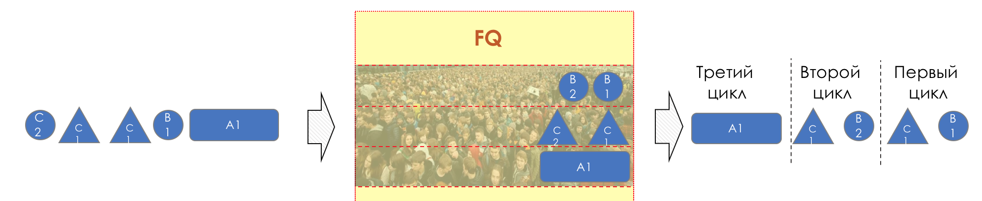
Here you can see that due to the large packet size in the 3rd queue, in the first two cycles, one of the first two packets was processed.
The description of the mechanisms of bit-by-bit Round Robin and GPS is already beyond the scope of this article, and I refer the reader to an independent study .
The second and partly the third flaws of the FQ attempted to close the WFQ, promulgated in 1989.
Each queue was given weight and, accordingly, the right for one cycle to give traffic a multiple of weight.
The weight was calculated on the basis of two parameters: the IP Precedence and then the packet length, which is still relevant then.
In the context of WFQ, the more weight, the worse.
Therefore, the higher the IP Precedence, the lower the packet weight.
The smaller the package size, the less and its weight.
Thus, high-priority packets of a small size receive the most resources, while low-priority giants wait.
In the illustration below, the packages received such weights that first one package from the first stage is skipped, then two from the second, again from the first, and only then the third is processed. For example, it could happen if the size of the packets in the second queue is relatively small.

About the harsh machinery of WFQ, with its packet finish time, virtual time and the Wig Theorem, you can read in a curious color document .
However, this did not solve the first and third problems. The flow based approach was just as inconvenient, and streams requiring short delays and stable jitters did not receive them.
This, however, did not prevent WFQ from finding use in some (mostly old) Cisco devices. There were up to 256 queues in which threads were placed based on the hash from their headers. A sort of compromise between the flow-based paradigm and limited resources.
Calling on the problem of complexity made CBWFQ with the arrival of DiffServ. Behavior Aggregate classified all categories of traffic into 8 classes and, accordingly, queues. This gave it a name and greatly simplified queuing service.
Weight in CBWFQ has acquired a different meaning. Weight was assigned to classes (not streams) manually in the configuration as desired by the administrator, because the DSCP field was already used for classification.
That is, the DSCP determined in which queue to place, and the configured weight - how many bands are available for this queue.
Most importantly, it indirectly made life and low-latency flows, which were now aggregated into one (two, three, ...) queues, and received their finest hour much more often. Life has become better, but still not good - there are no guarantees, in general, in the WFQ, everyone is still equal in terms of delays.
And the need to constantly monitor the size of packages, their fragmentation and defragmentation, has not gone away.
The final approach, the culmination of the bit-by-bit approach, is the integration of CBWFQ with PQ.
One of the queues becomes so-called LLQ (a queue with low latency), and while all the other queues are being processed by the CBWFQ controller, the PQ controller is running between the LLQ and the others.
That is, while there are packets in the LLQ, the remaining queues are waiting for their delays to grow. As soon as the packets in the LLQ ran out, they went to process the rest. There were packages in LLQ - they forgot about the rest, returned to him.
Inside LLQ, FIFO also works, so you shouldn’t shove anything there, no matter how you get, increasing buffer utilization and at the same time delays.
And yet, so that non-priority lines do not go hungry, in the LLQ it is worth setting a limit on the lane.

Here and the sheep are fed and the wolves are intact.
Hand in hand with FQ went and RR .
One was honest, but not simple. The other is quite the opposite.

RR went through the queues, extracting an equal number of packets from them. The approach is more primitive than FQ, and therefore unfair with respect to various threads. Aggressive sources could easily flood a strip of 1,500-byte packets.
However, it was very simple to implement - you do not need to know the size of the packet in the queue, fragment it and then collect it back.
However, his injustice in the distribution of the band blocked his way to the world - in the world of networks, a pure Round-Robin was not implemented.
The same fate and the WRR, which gave weight to the queues based on IP Precedence. In WRR, not an equal number of packets was taken out, but a multiple of the queue weight.
It would be possible to give more weight to queues with smaller packets, but this was not dynamically possible to do.

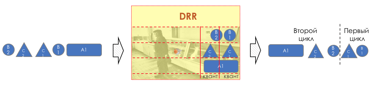
And suddenly, an extremely curious approach was proposed in 1995 by M. Shreedhar and G. Varghese.
Each queue has a separate credit line in bits.
When passing from the queue, as many packages are issued as long as there is enough credit.
The size of the package that is in the queue head is deducted from the loan amount.
If the difference is greater than zero, this packet is removed and the next one is checked. So until the difference is less than zero.
Even if the first package does not have enough credit, well, alas, seljava, it remains in the queue.
Before the next pass, the credit of each line is increased by a certain amount, called a quantum .
For different queues, the quantum is different - the larger the band to give, the larger the quantum.
Thus, all queues receive a guaranteed band, regardless of the size of the packets in it.
I would not understand from the explanation above how it works.
With the DWRR, the question still remains with the guarantee of delays and jitter - its weight does not solve it at all.
Theoretically, here you can do as with CB-WFQ, adding LLQ.
However, this is just one of the possible scenarios for the popularity of today.
Actually, PB-DWRR - Priority Based Deficit Weighted Round Robin is becoming almost mainstream today.
This is the same old evil DWRR, to which one more queue has been added - a priority queue, in which packets are processed with a higher priority. This does not mean that it is given a larger band, but the fact that packages will be taken from there more often.
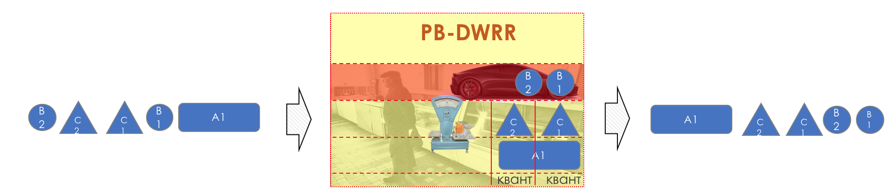
There are several approaches to implementing PB-DWRR. In some of them, as in PQ, any packet arriving at the priority queue is immediately withdrawn. In others, it is accessed every time a controller moves between queues. Thirdly, a credit and a quantum are introduced for it, so that the priority queue could not squeeze the entire strip.
Of course, we will not analyze them.
For decades, mankind has tried to solve the most difficult problem of providing the necessary level of service and fair distribution of the strip. The main tool was queues, the only question was how to pick up packets from the queues, trying to push them into one interface.
Starting with the FIFO, it invented the PQ - the voice was able to coexist with surfing, but there was no speech about the guarantee of the band.
There were several monstrous FQ, WFQ, which worked, if not per-flow, then almost like that. CB-WFQ came to a class society, but did not make it any easier.
As an alternative to him, RR developed. It turned into a WRR, and then a DWRR.
And in the depths of each dispatcher lives FIFO.
However, as you can see, there is not some kind of universal dispatcher, which handled all classes as they require. This is always a combination of controllers, one of which solves the problem of providing delays, jitter and no loss, and the other band allocation.
CBWFQ + LLQ or PB-WDRR or WDRR + PQ.
On real equipment, you can specify which queues to process by which dispatcher.
CBWFQ, WDRR and their derivatives are today's favorites.
PQ, FQ, WFQ, RR, WRR - we do not grieve or remember (unless, of course, we are preparing for the CCIE Clipper).
So, dispatchers are able to guarantee speed, but how to limit it from above?
The need to limit the speed of traffic at first glance is obvious - do not let the client out of the limits of his band according to the contract.
Yes. But not only. Suppose there is a 620 Mb / s RRL span connected via a 1Gb / s port. If the whole gigabit is shot at him, then somewhere on the RRL, which, quite likely, has no idea about queues and QoS, monstrous drops of a random nature will start, not tied to the real priorities of the traffic.
However, if you enable shaping up to 600 Mb / s on the router, then EF, CS6, CS7 will not be discarded at all, and in the BE, AFx, the band and the drops will be distributed according to their weights. Up to RRL will reach 600 MB / s and we will get a predictable picture.
Another example is the admission control. For example, two operators have agreed to trust all the markings of each other, except CS7 - if something has come to CS7 - discard. For CS6 and EF - to give a separate queue with a guarantee of delay and no loss.
But, what if the ingenious partner began to pour torrents into these lines? Goodbye telephony. And the protocols will most likely begin to fall apart.
It is logical in this case to agree with the partner about the band. All that fits into the contract - skip. What does not fit - discarded or transferred to another queue - BE, for example. Thus we protect our network and our services.
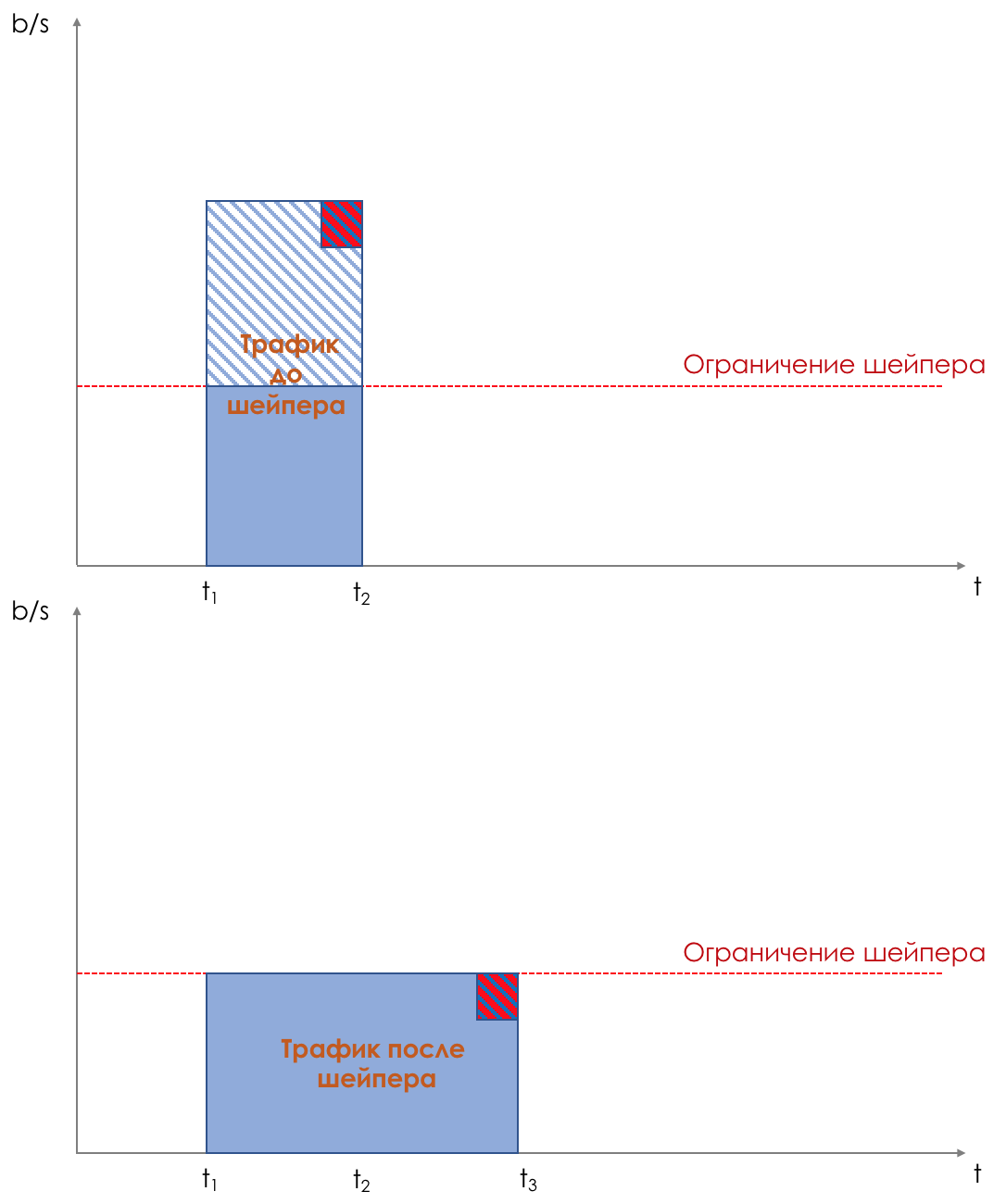
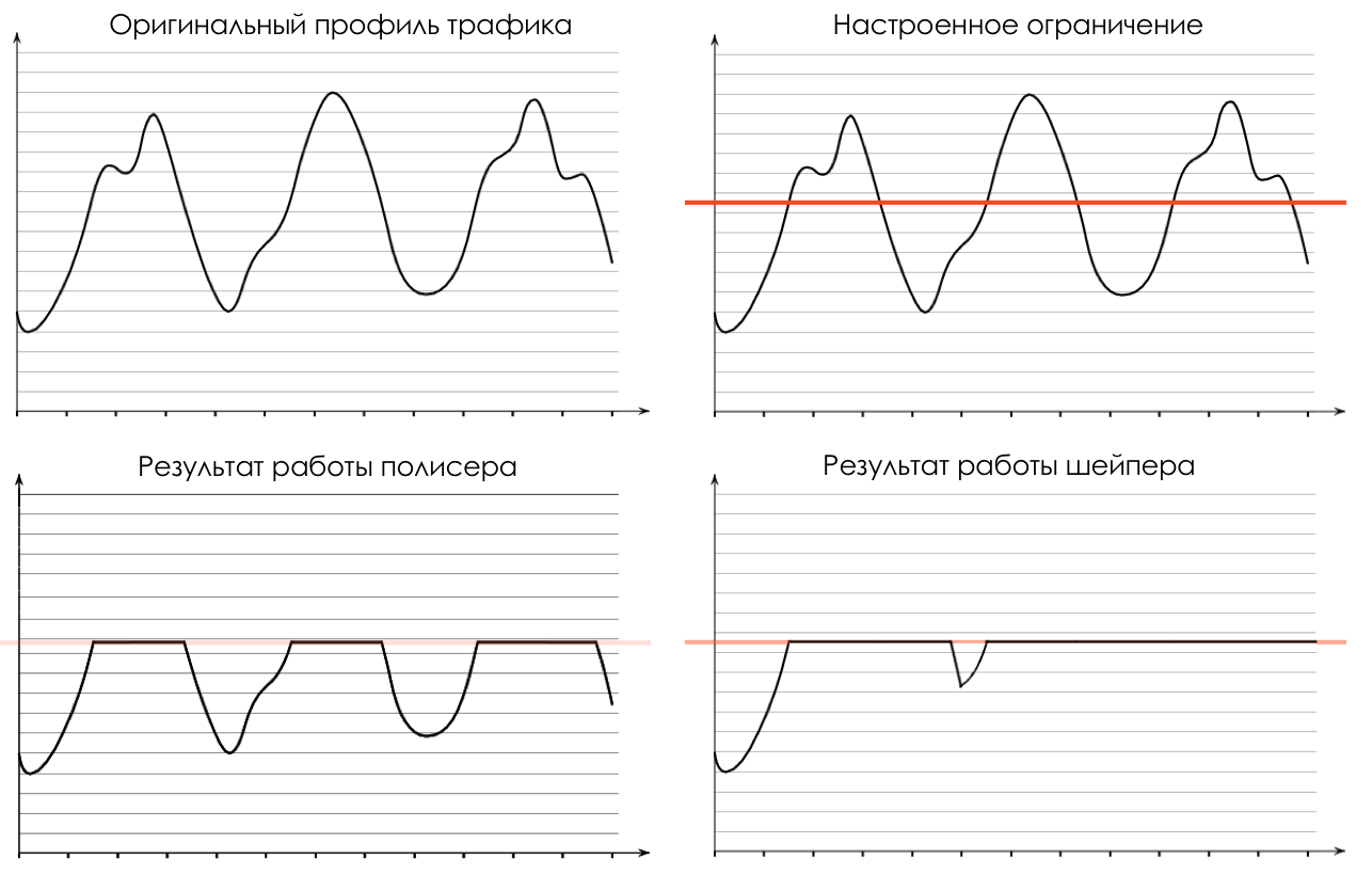
There are two fundamentally different approaches to speed limiting: polishing and shaping. They solve one problem, but in different ways.
Consider the difference on the example of such a traffic profile:

Polising limits the speed by dropping excess traffic.
Anything that exceeds the set value, policer cuts and throws.

What is cut is forgotten. The picture shows that the red packet is not in traffic after the polisher.
And this is how the selected profile will look like after the polisher:

Because of the rigor of the measures taken, this is called Hard Policing .
However, there are other possible actions.
Polyser usually works in conjunction with a traffic meter. The meter paints packages, as you remember, in green, yellow or red.
And on the basis of this color, the policer may not discard the package, but place it in another class. These are soft measures - Soft Policing .
It can be applied to both incoming traffic and outgoing traffic.
A distinctive feature of a polisher is its ability to absorb traffic spikes and determine the peak allowable speed due to the Token Bucket mechanism.
That is, in fact, everything that is above a given value is not cut off - it is allowed to go a little beyond it - short-term bursts or small excesses of the selected band are skipped.
The name “Policing” is dictated by a rather strict attitude of the tool to excess traffic - dropping or de-lowering to a lower class.
Shaping limits speed by buffering excess traffic.
All incoming traffic passes through the buffer. A shaper removes packets from this buffer at a constant rate.
If the speed of packet arrival to the buffer is below the output, they do not linger in the buffer - they fly through.
And if the rate of receipt is higher than the output, they begin to accumulate.
The output speed is always the same.
Thus, bursts of traffic are buffered and will be sent when it comes to their turn.
Therefore, along with scheduling in queues, shaping is the second tool contributing to the aggregate latency .
The illustration clearly shows how a packet arriving at the time t2 buffer appears at the output at time t3. t3-t2 is the delay introduced by the shaper.
Shaper is usually applied to outgoing traffic.
This is the profile after the shaper.
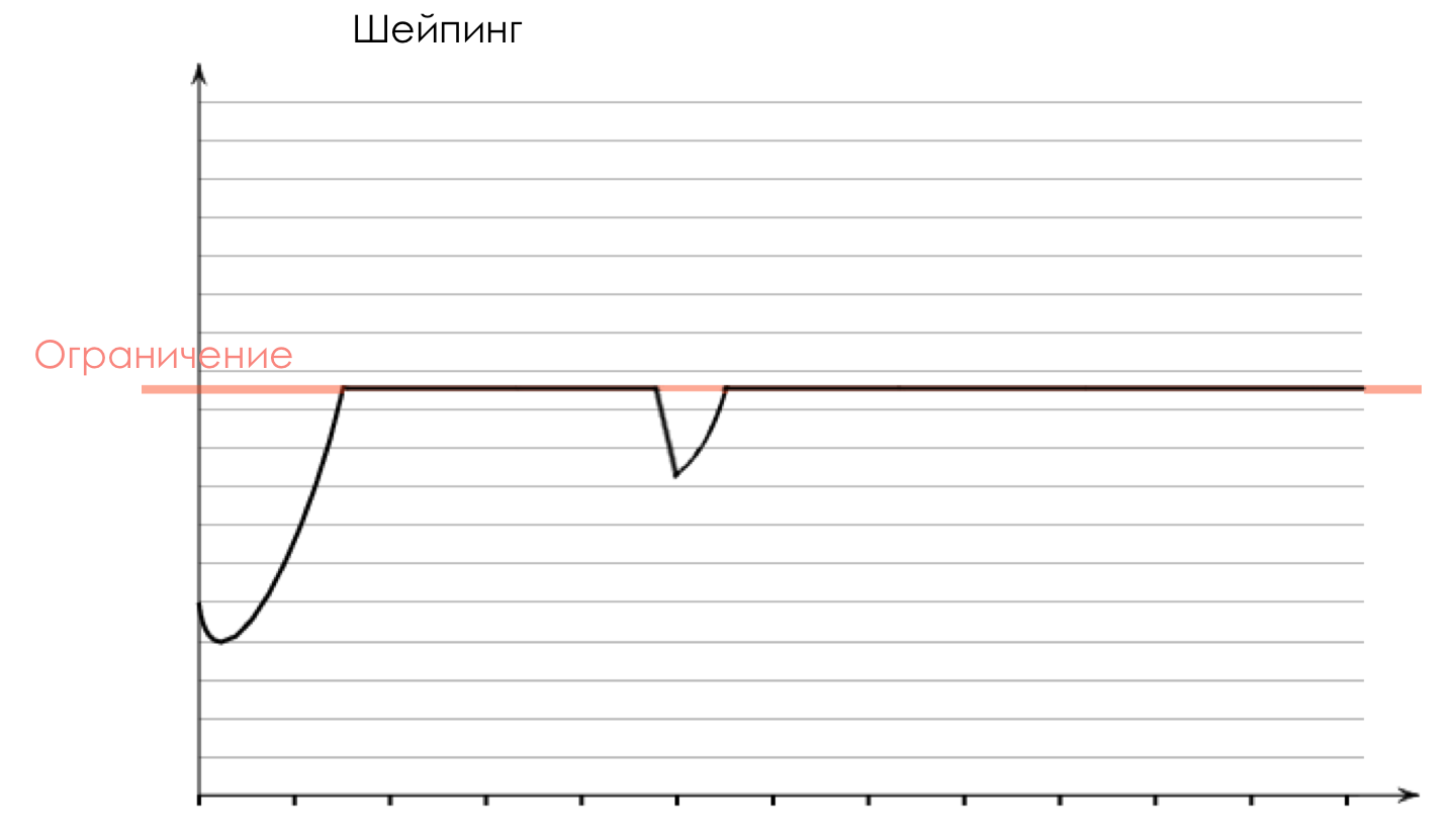
The name “Shaping” indicates that the tool gives shape to the traffic profile, smoothing it out.
The main advantage of this approach is the optimal use of the available band - instead of dropping excessive traffic, we postpone it.
The main drawback - the unpredictable delay - when filling the buffer, the packets will languish in it for a long time. Therefore, shaping is not suitable for all types of traffic.
Shaping uses the Leaky Bucket mechanism.
The work of a polisher is similar to a knife, which, moving along the surface of the oil, cuts off the sharp side of the tubercle.
The work of the shaper is like a roller, which smoothes the tubercles, distributing them evenly over the surface.
Shaper tries not to drop packets while they are being buffered at the cost of increasing latency.
Polysser does not introduce delays, but more readily discards packets.
Applications that are not sensitive to delays, but for which losses are undesirable, should be limited to a shaper.
For those for whom a late packet is like a lost one, it is better to drop it immediately - then polysing.
Shaper does not affect packet headers or their fate outside the node, while after polishing, the device can remake the class in the header. For example, the packet had an AF11 class at the entrance, the metering colored it yellow inside the device, it remarked its class at AF12 at the exit — on the next node it will have a higher drop probability.
The scheme is the same:
Configuration file. We
see this picture without applying restrictions:

We will proceed as follows:
Let's start with the shaper on Linkmeup_R4 .
Match all:
Shape to 20Mb / s:
Apply to the output interface:
All that must leave (output) interface Ethernet0 / 2, shape up to 20 Mb / s.
Shaper configuration file.
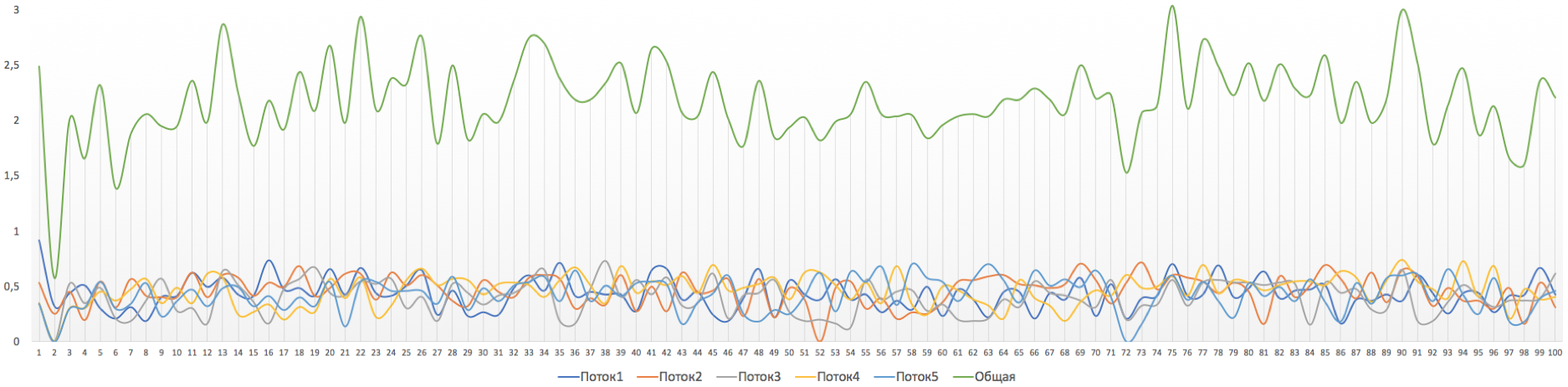
And here is the result:
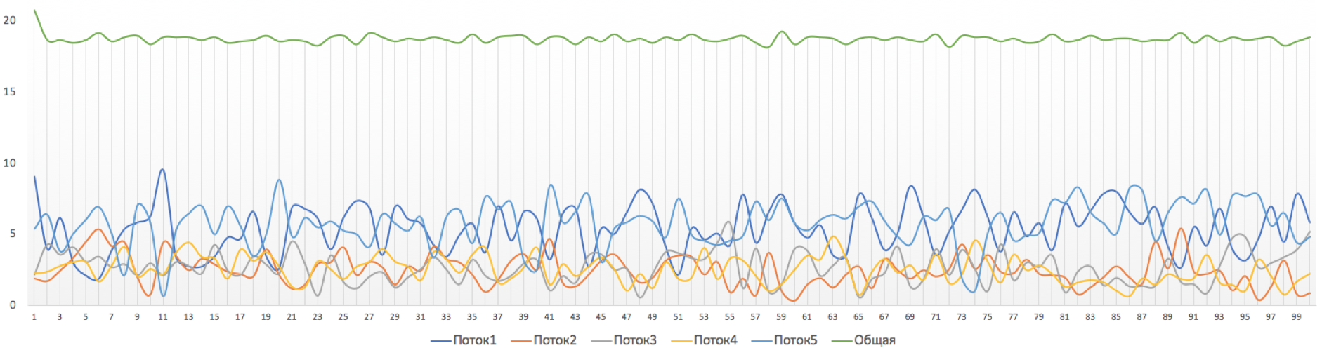
A fairly smooth line of total throughput and ragged graphics for each individual stream is obtained.
The fact is that we limit the overall lane with the shaper. However, depending on the platform, individual streams can also be individually shaped, thus obtaining equal opportunities.
Now let's set up polishing for Linkmeup_R2.
We will add a policer to the existing policy.
The interface policy has already been applied:
Here we indicate the average allowed speed of CIR (10Mb / s) and the allowed burst of Bc (1,875,000 bytes about 14.6 MB).
Later, explaining how the polisher works, I will tell you what CIR and Bc are and how to determine these values.
Polyser configuration file.
This picture is observed with polising. Immediately see dramatic changes in the level of speed:
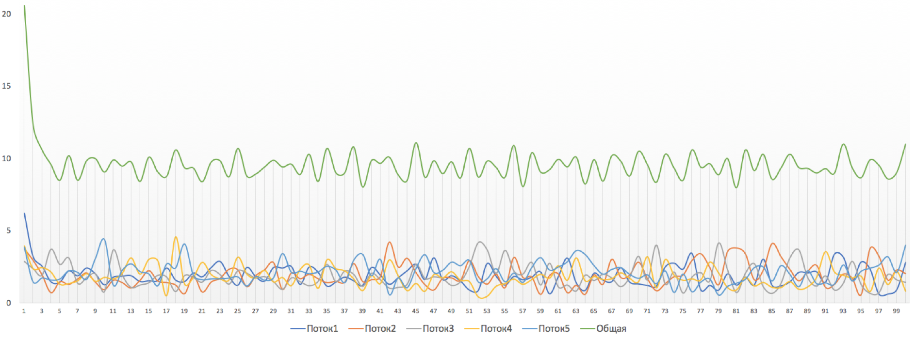
But such a curious picture is obtained if we make the allowable burst size too small, for example, 10,000 bytes.
The overall speed immediately dropped to about 2Mb / s.
Be careful with setting up the bursts :)
Test table.
It sounds easy and understandable. But how does it work in practice and is it implemented in hardware?
Example.
Is the limit of 400 MB / s a lot (or a little)? On average, the client uses only 320. But sometimes it rises to 410 for 5 minutes. And sometimes up to 460 for a minute. And sometimes up to 500 for half a second.
As a contractual provider, linkmeup can say - 400 and that's that! Want more, connect to the tariff 1Gb / s + 27 anime channels.
And we can increase customer loyalty, if it does not interfere with others by allowing such bursts.
How to allow 460Mb / s for just one minute, not 30 or forever?
How to allow 500 MB / s, if the band is free, and press up to 400, if there are other consumers?
Now take a break, pour a strong bucket.
Let's start with a simpler mechanism used by the shaper - a flowing bucket.
Leaky Bucket is a leaking bucket.

We have a bucket with a hole of a given size at the bottom. Packages are poured into this bucket on top. And from the bottom they flow with a constant bit rate.
When the bucket fills, new packages begin to be discarded.
The hole size is determined by the specified speed limit, which for Leaky Bucket is measured in bits per second.
The volume of the bucket, its fullness and output speed determine the delay introduced by the shaper.
For convenience, the bucket volume is usually measured in ms or μs.
In terms of implementation, Leaky Bucket is a regular SD-RAM based buffer.
Even if the shaping is not explicitly configured, in the presence of bursts that do not pass into the interface, the packets are temporarily added to the buffer and transmitted as the interface is released. This is also shaping.
Leaky Bucket is used only for shaping and is not suitable for poliscing.
Many believe that Token Bucket and Leaking Bucket are one and the same. Stronger was only Einstein's fault, adding the cosmological constant.
Switching chips are not very well aware of what time is, they consider even worse how many bits they transmitted per unit of time. Their job is to thresh.
Is this approaching bit another 400,000,000 bits per second, or is it already 400,000,001?

ASIC developers had a non-trivial engineering challenge.
She was divided into two subtasks:
The algorithm that solves the second problem is called Token Bucket. His idea is elegant and simple (no).
The task of Token Bucket is to allow traffic if it fits within the limit and discard / dye red if not.
At the same time, it is important to allow bursts of traffic, as this is normal.
And if in Leaky Bucket the bursts were absorbed by the buffer, then Token Bucket does not buffer anything.
Do not pay attention to the name yet =)
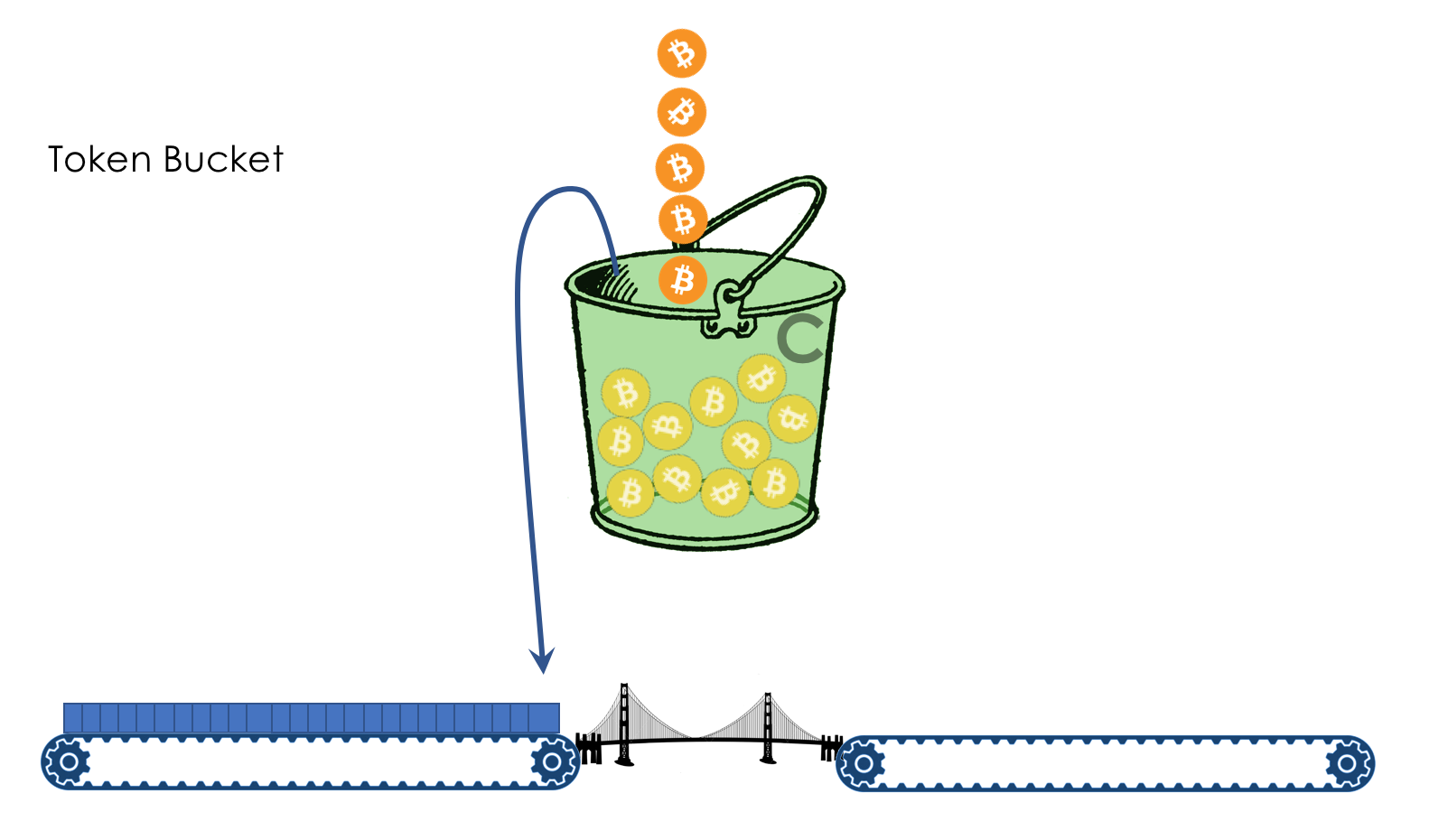
We have a bucket in which coins fall at a constant speed - 400 mega-coins per second, for example.
The volume of the bucket is 600 million coins. That is, it is filled in a half second.
Nearby are two conveyor belts: one brings packages, the second - takes away.
To get on the conveyor belt, the package must pay.
Coins for this he takes from the bucket in accordance with its size. Roughly speaking - how many bits - so many coins.

If the bucket is empty and the package is not enough coins, it is painted in red signal color and discarded. Alas, mudflows. At the same time, coins are not removed from the bucket.
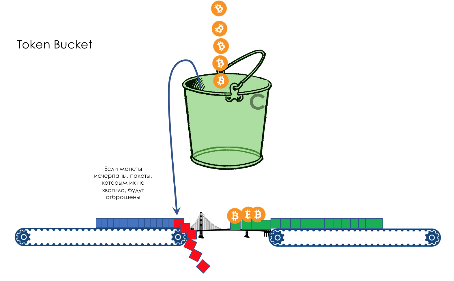
The next package of coins may already be enough - firstly, the package may be smaller, and, secondly, more coins will attack during this time.
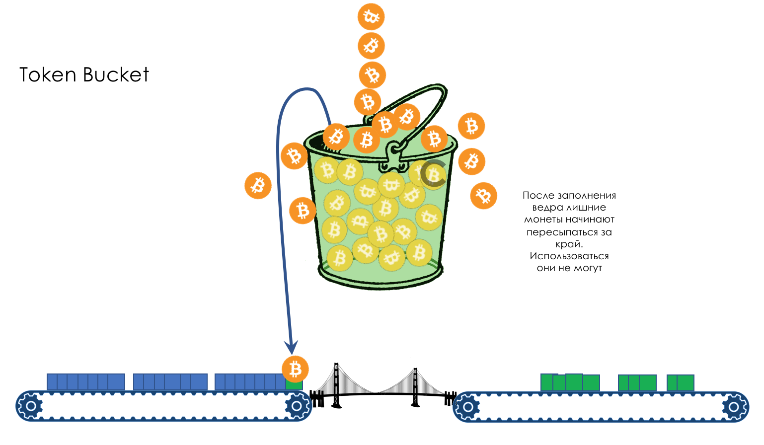
If the bucket is already full, all new coins will be thrown away.
It all depends on the rate of arrival of packages and their size.
If it is consistently lower than or equal to 400 MB per second, then there will always be enough coins.
If higher, then some packets will be lost.
For example, a stable stream of 399 MB / s for 600 seconds will allow the bucket to fill to the brim.
Further, traffic can go up to 1000Mb / s and stay at this level for 1 second - 600 Mm (Megamonet) of the stock and 400 Mm / s of the guaranteed band.
Or the traffic can rise up to 410 Mb / s and stay that way for 60 seconds.
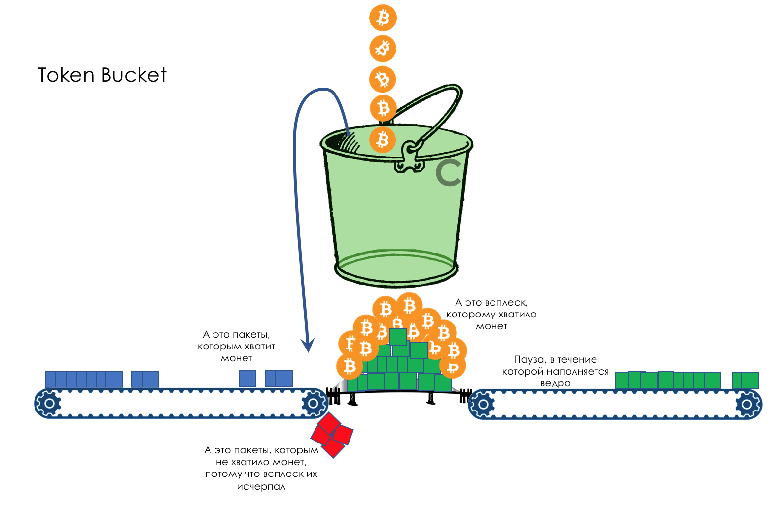
That is, the stock of coins allows you to slightly go beyond the limit for a long time or throw out a short but high burst.
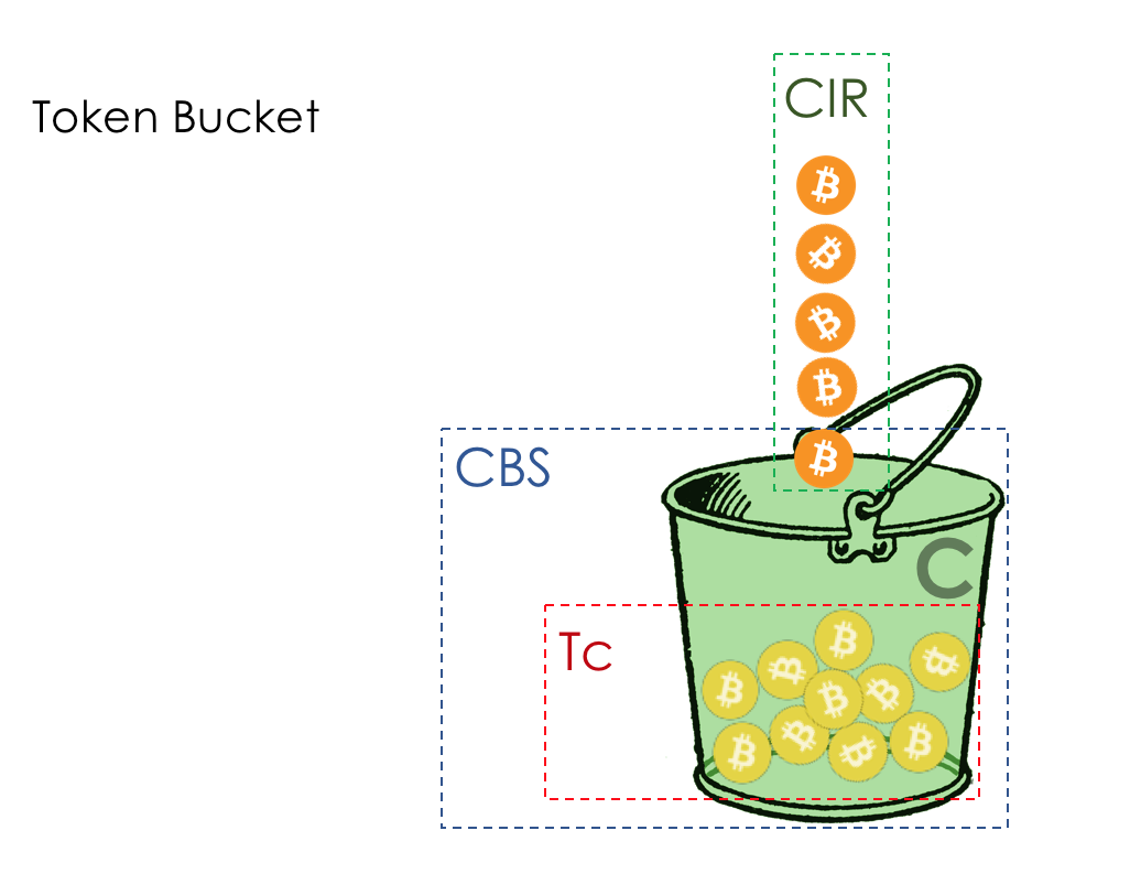
Now to the terminology.
The rate of arrival of coins in a bucket - CIR - Committed Information Part Rate (Guaranteed average speed). Measured in bits per second.
The number of coins that can be stored in a bucket - CBS - Committed Burst Size . Maximum allowed burst size. Measured in bytes. Sometimes, as you may have noticed, is called Bc .
Tc - The number of coins (Token) in the C bucket (CBS) at the moment.
Single Rate means that there is only one average allowed speed, and Two Color - that you can paint traffic in one of two colors: green or red.
Used for polysing in PHB CS and EF, where speeding is not expected, but if it happens, it is better to drop it immediately.
Further we will consider more difficult: Single Rate - Three Color.
The disadvantage of the previous scheme is that there are only two colors. What if we do not want to discard everything that is above the average allowed speed, but want to be even more loyal?
the TCM-sr ( Single Rate - the Three the Color The Marking ) enters the second bucket in - E . At this time, the coins are not placed in a bucket filled with the C , are poured into E . EBS is
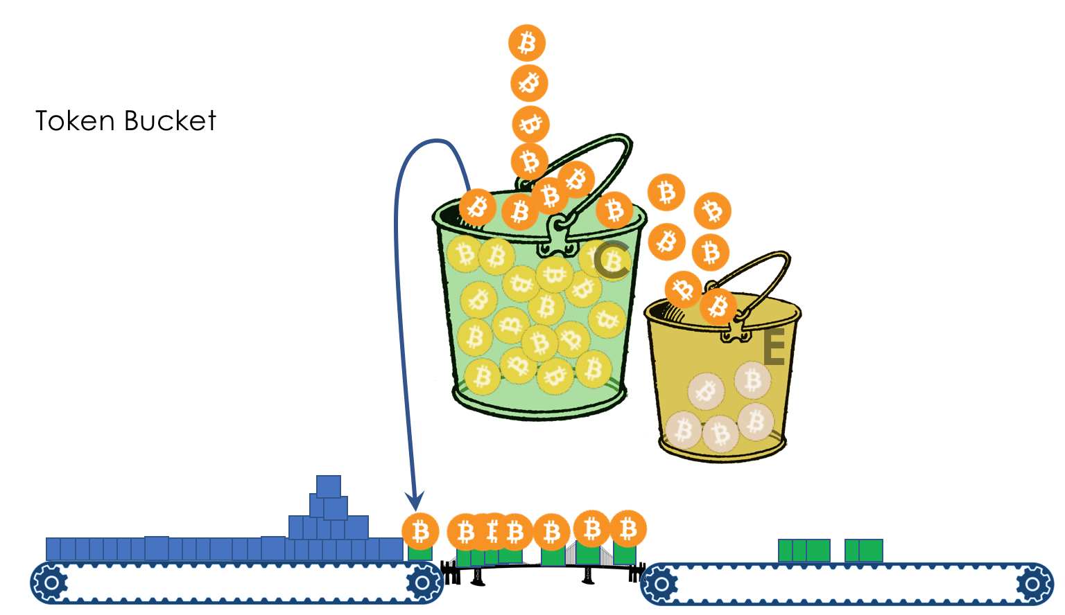
added to CIR and CBS - Excess Burst Size - The allowed burst size during peaks. Te - the number of coins in a bucket E .

Suppose a package of size B came through the pipeline. Then
Please note that for a specific package Tc and Te are not cumulative .
That is, a packet of 8000 bytes in size will not pass, even if there are 3000 coins in the C bucket and 7000 coins in the E. There is not enough in C , in E there is not enough - we put a red stamp - shurui from here.
This is a very elegant scheme. All traffic that fits into the average CIR + CBS limit (the author knows that it is impossible to directly add bits / s and bytes) - goes green. At peak times when the customer has exhausted the coins in the C bucket , he still has the stock of Te in the E bucket accumulated during the downtime .
That is, you can skip a little more, but in the case of congestion, these are more likely to be discarded.
sr-TCM is described in RFC 2697 .
Used for polysing in PHB AF.
Well, the last system is the most flexible and therefore complex - Two Rate - Three Color.
The Tr-TCM model was born from the idea that, not to the detriment of other users and types of traffic, why shouldn't the client be given a bit more pleasant opportunities, and even better to sell.
Let's tell him that he is guaranteed 400 Mb / s, and if there are free resources, then 500. Are you ready to pay 30 rubles more?
Added another bucket P .
Thus:
CIR - guaranteed average speed.
CBS is the same allowed burst size (bucket volume C ).
PIR - Peak Information Rate - the maximum average speed.
EBS is the allowed burst size during peaks (Bucket Volume P ).
Unlike sr-TCM, tr-TCM now in both buckets are independently received coins. In C - with CIR speed, in P - PIR.
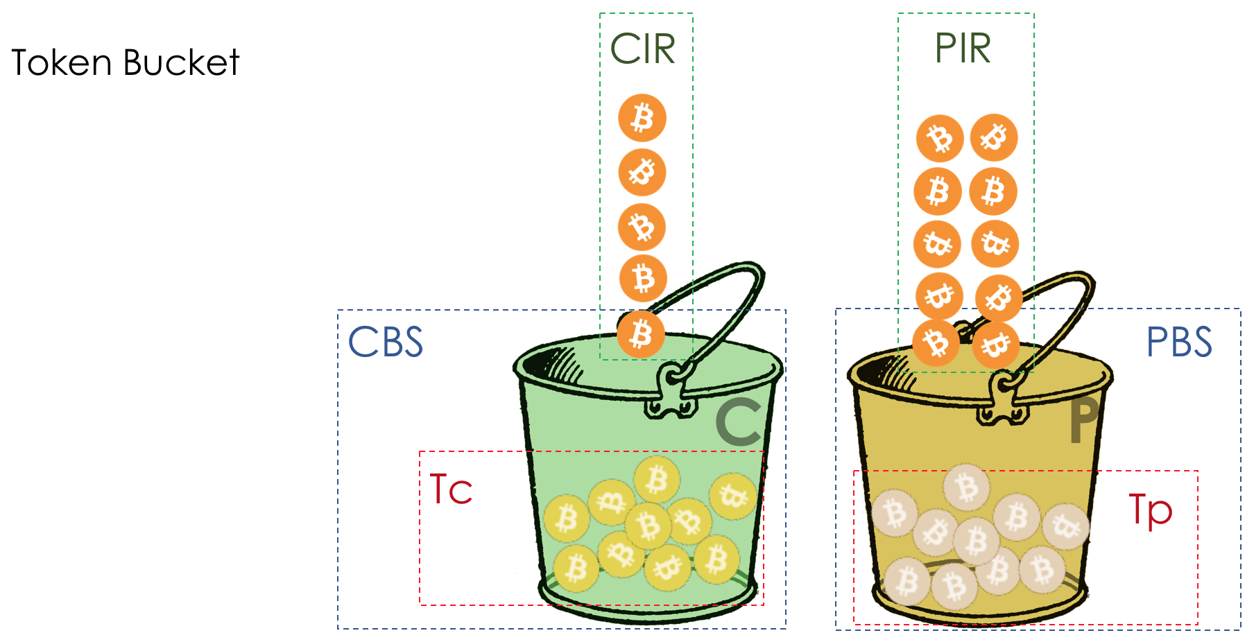
Which rules?
A b- byte packet arrives .

That is, the rules in tr-TCM are different.
As long as traffic keeps within guaranteed speed, coins are taken out of both buckets. Due to this, when the coins run out in the C bucket , they will remain in P , but just enough to not exceed the PIR (if it were taken out only from C , then P would fill more and give a much higher speed).
Accordingly, if it is higher than guaranteed, but lower than the peak, coins are removed only from P , because there is already nothing in C.
tr-TCM monitors not only bursts, but also constant peak speed.
tr-TCM is described in RFC 2698 .
Also used for polysing in PHB AF.
While shaping puts off traffic when it is exceeded, polishing discards it.
Shaping is not suitable for applications that are sensitive to delays and jitter.
To implement polishing in hardware, the algorithm is Token Bucket, for shaping - Leaky Bucket.
Token Bucket can be:
sr-TCM focuses on traffic over limit. tr-TCM - at the rate at which it arrives.
Polising can be used on the input and output from the device. Shaping mainly at the exit.
For PHB CS and EF, Single Rate Two Color Marking is used.
For AF, sr-TCM or tr-TCM.
For perhaps a better understanding, I recommend turning to the original RFC or reading here .
Above, I described all the basic QoS mechanisms, if not to go into hierarchical QoS. The most complex system with numerous moving parts.
Everything is good (right?) It has sounded so far, but what is happening under the vanilla outer panel of the router?
Over the years, vendors added more and more konutry, developed sophisticated chips, expanded buffers to keep pace with the growing volume of traffic and its new categories, on the one hand, and to solve the growing problems caused by the first item, on the other.
Continuing race. You can not lose packages if a competitor does not lose them. You can not abandon the functionality if the opponent is with him under the doors of the customer.
Ida in the lair of proprietary!
In this chapter, I take on the ungrateful task. If you describe as simple as possible, there will always be those who say that everything is not so in reality.
If you describe it as it is, the reader will drop the article, because it will turn into a drawing of a submarine, more precisely the drawings of three boats with pencils of different colors on one sheet.
In general, I will make a disclaimer that in reality everything is not as it really is, and will follow the simple version.
Forgive me, my companion perfectionist.
What controls the behavior of the node and starts the appropriate mechanisms in relation to the package? The priority that he carries in one of the headers? Yes and no.

As mentioned above, a standard switching header usually ceases to exist within a network device.

As soon as the packet has got on the switching chip, the headers are removed from it and sent for analysis, and the payload is languishing in some kind of temporary buffer.
Based on the headers, a classification occurs (BA or MF) and the decision to transfer is made.
In an instant, an internal header with package metadata is attached to the packet.
This metadata carries a lot of important information - the sender and recipient addresses, the output chip, the cell sequence number, if there was packet fragmentation and necessarily class marking (CoS) and drop priority (Drop Precedence). Only marking in the internal format - it may or may not coincide with the DSCP.
In principle, inside the box you can set an arbitrary length of the marking, not being tied to the standards, and determine very flexible actions with the package.
At Cisco, the internal labeling is called QoS Group, at Juniper - Forwarding Class, Huawei has not decided: it calls internal priorities, somewhere local priorities, Service-Class somewhere, and CoS somewhere. Add in comments names for other vendors - I will add.
This internal marking is assigned based on the classification that the node has performed.
It is important that if not stated otherwise, the internal marking only works inside the node, but then it doesn’t appear on the label in the headers of the packet that will be sent from the node - it will remain the same.
However, at the entrance to the DS-domain after classification, a remarking into a certain class of service adopted in this network usually occurs. Then the internal marking is converted to the value adopted for this class on the network, and is written in the header of the packet being sent.
The internal marking of CoS and Drop Precedence only defines the behavior inside this node and is not explicitly passed on to its neighbors, except for remarking the headers.
CoS and Drop Precedence determine the PHB, its mechanisms and parameters: overload prevention, congestion management, dispatching, remarking.
Through what circles pass the packets between the input and output interfaces I discussed in the previous article . Actually, it turned out to be unplanned, since at some point it became obvious that it was premature to talk about QoS without an understanding of the architecture.
However, let's repeat.
In this case, the router must solve a complex equation.
Spread out all the classes, provide someone with a wide band, someone low latency, someone to ensure the absence of losses.
And at the same time have time to skip all traffic if possible.
In addition, you need to do shaping, possibly polishing. If suddenly there is an overload, then cope with it.
And that's not counting Lukap, processing ACL, statistics calculation.
Unenviable share. But robots are driving, not man.
In fact, there are only two places where the QoS mechanisms work - the switching chip and the traffic management / queue chip.
At the same time on the switching chip, operations occur that require analysis or actions with headers.
The rest is taken by TM. These are mainly routine operations with a predefined algorithm and adjustable parameters:
TM is a smart buffer, usually based on SD-RAM.
He is smart because, a) programmable, b) with queues he knows how to do all sorts of tricky things.
It is often distributed — SD-RAM chips are located on each interface board, and together they combine into a VOQ (Virtual Output Queue) that solves the problem Head of Line Blocking.
The fact is that if the switching chip or the output interface is flooded, then they ask the input chip to slow down and not send traffic for some time. If there is only one queue in all directions, then it is very disappointing that all the others suffer from one output interface. This is the Head of Line Blocking.
VOQ creates multiple virtual output queues for each existing output interface on the input interface board.
Moreover, these lines in modern equipment take into account the labeling of the package.
About VOQ described in sufficient detail in a series of notes here .
By the way, the lines are actually placed, they are promoted, not the packages themselves, but only the records about them, are being withdrawn, etc. It makes no sense to do so many gestures with large arrays of bits. While QoS is being measured over the records, the packets are fine in the memory and retrieved from there to the address.
VOQ is a software queue (the English term Software Queue is more accurate). After it, immediately before the interface there is also a hardware queue, which always, strictly works on FIFO. It’s almost impossible to control any of its parameters (for example, Cisco allows you to adjust only the depth using the tx-ring-limit command).
Just between the software and hardware queue, you can run arbitrary dispatchers. It is in the program queue that Head / Tail-drop and AQM, polishing and shaping work.
The size of the hardware queue is very small (units of packages), because the dispatcher does all the work of placing in the line-rate.
Unfortunately, you can make a lot of reservations here, and in general, cross out everything with a red pen and say “it’s not like that with vendor X”.
I would like to make one more remark about service packages. They are handled differently than transit user packets.
Being generated locally, they are not checked for compliance with ACL rules and speed limits.
The packets from the outside, destined for the CPU, from the output switching chip fall into other queues — to the CPU — based on the protocol type.
For example, BFD has the highest priority, OSPF can wait a little longer, and ICMP and generally not afraid to drop. That is, the more important the packet is for network performance, the higher its class of service is when sending to the CPU. That is why seeing in ping or tracing varying delays on transit hops is normal - ICMP is not a priority for CPU traffic.
In addition, protocol packets applyCoPP - Control Plane Protection (or Policing) - speed limits to avoid high CPU utilization - again, better predictable drops in low priority queues before problems start.
CoPP will help from both targeted DoS and abnormal network behavior (for example, loops) when a lot of broadcast traffic begins to arrive on the device.
This release has had many reviewers.
Thank.
Alexander Fatinu ( LoxmatiyMamont ) for introductory words and valuable tips on the expressiveness and clarity of the text.
Alexander Clipper (@ metallicat20) for peer review.
Alexandru Klimenko (@ v00lk) for harsh criticism and the most massive changes in recent days.
Andrei Glazkov (@glazgoo) for comments on structure, terminology and commas.
Artem Chernobay for KDPV.
Anton Klochkov (@NAT_GTX) for contacts with Miran.
Miran (miran.ru) for organizing a server with Eve and broadcast. Traditionally, my family, which, incidentally, this time suffered the least because of her absence next to the most difficult moments.
And here we come to the topic of QoS.
Do you know why only now and why this will be the closing article of the entire course of SDCM? Because QoS is unusually complex. The hardest thing that was previously in the cycle.
This is not some kind of magic archiver, which will cleverly compress traffic on the fly and push your gigabit into a one-megabyte uplink. QoS is about how to sacrifice something unnecessary, cramming nevpihuemoe within the limits of what is permitted.
QoS is so enmeshed with the aura of shamanism and inaccessibility that all young (and not only) engineers try to carefully ignore its existence, believing that it is enough to shower problems with money and endlessly expanding links. True, until they realize that with such an approach, failure inevitably awaits them. Either the business will start asking uncomfortable questions, or there will be a lot of problems almost unrelated to the width of the channel, but directly dependent on the effectiveness of its use. Yeah, VoIP is actively waving a handle from behind the scenes, and multicast traffic sarcastically strokes your back.
Therefore, let's just realize that QoS is necessary, it will have to get to know one way or another, and why not start now in a calm atmosphere.
Content
1. What determines QoS?
- Losses
- Delays
- Jitter
2. Three QoS models
- Best effort
- Integrated services
- Differentiated Services
3. DiffServ mechanisms
4. Classification and labeling
- Behavior Aggregate
- Multi-Field
- Interface-Based
5. Queues
6. Congestion Avoidance
- Tail Drop and Head Drop
- RED
- Wred
7. Congestion Management
- First In, First Out
- Priority queuing
- Fair queuing
- Round robin
8. Speed Limit
- Shaping
- Policing
- Leaky Bucket and Token Bucket Mechanisms
9. Hardware QoS implementation
Before the reader dives into this hole, I will lay three installations in it:
- Not all problems can be solved by expanding the band.
- QoS does not extend the bandwidth.
- QoS about managing limited resources.
1. What determines QoS?
The business expects from the network stack that it will simply perform its simple function well - to deliver the bitstream from one host to another: without loss and in a predictable time.
All network quality metrics can be derived from this short sentence:
- Losses
- Delays
- Jitter
These three characteristics determine the quality of the network regardless of its nature: packet, channel, IP, MPLS, radio, pigeons .
Losses
This metric tells how many of the packets sent by the source reached the addressee.
The cause of losses can be a problem in the interface / cable, network overload, bit errors, blocking ACL rules.
What to do in case of losses is decided by the application. It can ignore them, as in the case of a telephone conversation, where the late packet is no longer needed, or to re-request it to be sent - this is what TCP does to ensure accurate delivery of the original data.
How to manage losses, if they are inevitable, in the chapter Congestion Management.
How to use losses in the benefit in the chapter Prevention of overloads.
Delays
This is the time it takes the data to get from the source to the recipient.
The cumulative delay is made up of the following components.
- Delay Serialization ( Serialization the Delay ) - time during which the unit will decompose a package into bits, and put in a link to the next node. It is determined by the speed of the interface. So, for example, transmission of a packet of 1500 bytes in size through an interface of 100 Mb / s will take 0.0001 s, and for 56 Kb / s - 0.2 s.
- The delay in signal transmission in the medium ( Propagation Delay ) is the result of the notorious limitation of the speed of propagation of electromagnetic waves. Physics does not allow getting from New York to Tomsk on the surface of the planet in less than 30 ms (in fact, about 70 ms).
- The delays introduced by QoS are the languor of packets in queues ( Queuing Delay ) and the consequences of shaping ( Shaping Delay ). Today we will talk about this a lot and tediously in the chapter Speed control.
- The delay packet processing ( Processing the Delay ) - time to make a decision what to do with the package: lookup, ACL, NAT, DPI - and delivering it from the input to the output interface. But on the day when Juniper, in its M40, split Control and Data Plane, the processing delay became neglected.
Delays are not so terrible for applications where rush is not required: file sharing, surfing, VoD, Internet radio stations, etc. And on the contrary, they are critical for interactive: 200ms are already unpleasant to the ear during a telephone conversation.
A delayed term, but not synonymous with RTT ( Round Trip Time ), is a round-trip way. When pinging and tracing, you see RTT, and not one-way delay, although the values do have a correlation.
Jitter
The difference in delays between the delivery of consecutive packets is called jitter.
Like latency, jitter is irrelevant for many applications. And even it would seem, what's the difference - the package was delivered, what more?
However, it is important for interactive services.
Take as an example the same telephony. In fact, it is the digitization of analog signals divided into separate chunks of data. The output is a fairly uniform stream of packets. On the receiving side there is a small buffer of a fixed size, in which successively incoming packets are placed. To restore an analog signal, you need a certain number of them. Under conditions of floating delays, the next data chunk may not arrive in time, which is tantamount to loss, and the signal cannot be recovered.
The greatest contribution to the variability of the delay makes just QoS. About this, too, a lot and tedious in the same chapters of the speed limit.
These are the three main characteristics of the quality of the network, but there are two others that also play an important role.
Unordered delivery
A number of applications such as telephony, NAS , CES are extremely sensitive to unordered packet delivery when they arrive at the recipient in a different order than they were sent. This can lead to loss of connectivity, errors, damage to the file system.
Although unordered delivery is not a formal characteristic of QoS, it definitely refers to network quality.
Even in the case of TCP tolerant to this kind of problems, duplicate ACKs and retransmitts occur.
Bandwidth
It is not distinguished as the network quality metric, since in fact its lack results in the three indicated above. However, in our realities, when it should be guaranteed to some applications or, conversely, should be limited under the contract, for example MPLS TE reserves it throughout the entire LSP, it is worth mentioning it, at least as a weak metric.
Speed control mechanisms are discussed in chapters Speed limit.
Why characteristics may deteriorate?
So, we start with a very primitive view that a network device (whether it is a switch, a router, a firewall, or whatever) is just another piece of pipe called a communication channel, the same as a copper wire or an optical cable.
Then all the packages fly through in the same order in which they came and do not experience any additional delays - there is nowhere to linger.
But in fact, each router recovers bits and packets from the signal, does something with them (we do not think about it yet) and then converts the packets back into a signal.
A delay in serialization appears. But in general, it is not scary because it is constant. Not scary as long as the width of the output interface is larger than the input.
For example, at the entrance to the device is a gigabit port, and at the output is a radio relay line 620 MB / s connected to the same gigabit port?
Nobody forbids bullet through a formally gigabit link gigabit traffic.
There is nothing you can do - 380 MB / s will be spilled on the floor.
Here they are - the loss.
But at the same time, I would very much like to see the worst part of it spill out - the video from youtube, and the executive’s telephone conversation with the plant director wasn’t interrupted or even croaked.
I wish the voice had a dedicated line.
Or the input interfaces are five, and the output one, and at the same time, five nodes began to try to infuse traffic to one recipient.
Add a pinch of VoIP theory (an article about which no one has written) - it is very sensitive to delays and their variations.
If for a TCP stream of video from youtube (at the time of writing this article QUIC is still an experiment), even seconds are absolutely free of delays due to buffering, then the director will call the head of the technical department after the first such conversation with Kamchatka.
In older times, when the author of the cycle was still doing lessons in the evenings, the problem was particularly acute. Modem connections had a speed of 56k .
And when such a connection received a one-and-a-half-kilo packet, he occupied the entire line for 200 ms. No one else could pass at that moment. Vote? No, have not heard.
Therefore, the MTU issue is so important - the package should not occupy the interface for too long. The less speedy it is, the less MTU is needed.
These are the delays.
Now the channel is free and the delay is low, in a second someone started downloading a large file and the delays grew. Here it is - jitter.
Thus, it is necessary that voice packets fly through the pipe with minimal delays, and youtube will wait.
Available 620 MB / s should be used for voice, video, and B2B clients buying VPNs. I wish that one traffic did not oppress the other, then you need a band guarantee.
All the above characteristics are universal regarding the nature of the network. However, there are three different approaches to their provision.
2. Three QoS models
- Best Effort - no guarantee of quality. Everyone is equal.
- IntServ - quality assurance for each stream. Reserve resources from source to destination.
- DiffServ - there is no reservation. Each node determines how to ensure the desired quality.
Best Effort (BE)
No guarantees.
The simplest approach to the implementation of QoS, from which IP networks began and which is practiced to this day - sometimes because it is enough, but more often because no one thought about QoS.
By the way, when you send traffic to the Internet, it will be processed there as BestEffort. Therefore, through VPN, prokinutnye over the Internet (as opposed to VPN provided by the provider), can not very confident to go important traffic, such as a telephone conversation.
In the case of BE, all traffic categories are equal, no preference is given. Accordingly, there is no guarantee for delay / jitter or band.
This approach has a somewhat counterintuitive name - Best Effort, which is misleading the novice with the word “best”.
However, the phrase “I will do my best” means that the speaker will try to do everything that he can, but does not guarantee anything.
Nothing is required to implement BE — this is the default behavior. It is cheap in production, the personnel do not need deep specific knowledge, QoS in this case defies any adjustment.
However, this simplicity and static does not mean that the Best Effort approach is not used anywhere. It finds application in networks with high bandwidth and the absence of congestion and surges.
For example, on transcontinental lines or in networks of some data centers where there is no oversubscription.
In other words, in networks without overloads and where there is no need to treat any traffic in a special way (for example, telephony), BE is quite appropriate.
Intserv
Provisional reservation of resources for the stream from the source to the recipient.
In the growing unsystematic Internet, the fathers of the MIT, Xerox, ISI networks decided to add an element of predictability, while maintaining its efficiency and flexibility.
So in 1994, the idea of IntServ was born in response to the rapid growth of real-time traffic and the development of multicast. It was reduced then to IS.
The name reflects the desire in the same network to simultaneously provide services for real-time and non-real-time traffic types, providing, first of all, the priority right to use resources through band reservation. The possibility of reusing the band, on which everyone earns, and thanks to what the IP shot, at the same time remained.
The reservation mission was assigned to RSVP, which foreach stream reserves a band on each network device.
Roughly speaking, before setting up a Single Rate Three Color MarkerP session or starting data exchange, end hosts send an RSVP Path indicating the required bandwidth. And if RSVP Resv is back to both of them, they can start communicating. However, if there are no resources available, RSVP returns an error and the hosts cannot communicate or will follow the BE.
Let the bravest of readers now imagine that for any stream on the Internet today a channel will be signaled in advance. Consider that this requires non-zero CPU and memory costs for eachtransit node, postpones the actual interaction for some time, it becomes clear why IntServ was actually a stillborn idea - zero scalability.
In a sense, the modern incarnation of IntServ is MPLS TE with the RSVP version RSVP TE adapted for tag transmission. Although here, of course, not End-to-End and not per-flow.
IntServ is described in RFC 1633 .
The document is in principle curious to evaluate how naive one can be in forecasts.
Diffserv
DiffServ complex.
When it became clear at the end of the 90s that the IntServ IP end-to-end approach failed, the IETF convened in 1997 a working group, Differentiated Services, which developed the following requirements for a new QoS model:
- No alarm (Adyos, RSVP!).
- Based on aggregated traffic classification, instead of focusing on flows, clients, etc.
- It has a limited and deterministic set of actions for processing data traffic classes.
As a result, the epoch-making RFC 2474 ( Definition of the Differentiated Services Field (DS Field) in the IPv4 and IPv6 Headers ) and RFC 2475 ( An Architecture for Differentiated Services ) were born in 1998 .
And then all the way, we will only talk about DiffServ.
It should be noted that the name DiffServ is not the antithesis of IntServ. It reflects that we differentiate the services provided to various applications, or rather their traffic, in other words, we divide / differentiate these types of traffic.
IntServ does the same thing - it distinguishes between the types of BE traffic and Real-Time traffic transmitted on the same network. Both: both IntServ and DiffServ - refer to ways to differentiate services.
3. DiffServ mechanisms
What is DiffServ and why does it win against IntServ?
If it is very simple, then the traffic is divided into classes. A package at the entrance to each node is classified and a set of tools is applied to it, which processes packages of different classes differently, thus providing them with a different level of service.
But it just will not .
At the heart of DiffServ is the ideological concept of the IP traditionally held in the traditions of PHB - Per-Hop Behavior . Each node on the path of traffic independently makes a decision on how to behave relative to the incoming packet, based on its headers.
The actions of a packet router are called a behavior model ( Behavior). The number of such models is deterministic and limited. Cross-device behaviors in relation to the same traffic may be different, so they are per-hop.
The concepts of Behavior and PHB I will use in the article as synonyms.
There is a slight confusion. PHB is, on the one hand, a common concept of independent behavior of each node, on the other - a specific model on a particular node. With this we will understand.
The behavior model is determined by the set of tools and their parameters: Policing, Dropping, Queuing, Scheduling, Shaping.
Using existing behaviors, the network can provide various classes of service ( Class of Service ).
That is, different categories of traffic can get a different level of service on the network by applying different PHBs to them.
Accordingly, first of all, you need to determine which class of service the traffic belongs to - classification ( Classification ).
Each node independently classifies incoming packets.
After classification, a measurement occurs ( Metering ) - how many bits / bytes of the traffic of a given class has arrived at the router.
Based on the results, the packages can be colored ( Coloring ): green (within the limits of the established limit), yellow (outside the limit), red (all along the coast).
If necessary, further there is policing ( Policing ) (sorry for such a tracing paper, there is a better option - write, I will change). A polisher based on the color of the packet assigns an action to the packet — transfer, discard, or remarry.
After that, the packet should go into one of the queues ( Queuing ). For each class of service, a separate queue is allocated, which allows them to be differentiated using different PHBs.
But even before the packet enters the queue, it can be dropped ( dropper ) if the queue is full.
If he is green, he will pass, if yellow, then it is likely to be rejected, if the queue is full, and if red - this is a sure suicide bomber. Conventionally, the probability of dropping depends on the color of the packet and the fullness of the queue where it is going to go.
At the exit of the queue, the shaper ( Shaper ), whose task is very similar to the polisher problem, is to limit traffic to the specified value.
You can configure arbitrary shapers for individual queues or even within queues.
On the difference between the shaper and the polisher in the chapter Speed Limit.
All queues should eventually merge into a single output interface.
Remember the situation when on the road 8 lanes merge into 3. Without a traffic controller, this turns into chaos. Separating by queues would not make sense if we had the same output as the output.
Therefore, there is a special dispatcher ( Scheduler ), which cyclically takes out packets from different queues and sends it to the interface ( Scheduling ).
In fact, a bunch of queues and the dispatcher is the most important QoS mechanism that allows you to apply different rules to different traffic classes, one providing a wide band, the other low delays, the third the absence of drops.
Next, the packets already go to the interface, where the packets are converted into a bitstream — serialization ( Serialization ) and then the medium signal.
In DiffServ, the behavior of each node, regardless of the rest, there are no signaling protocols that would report which QoS policy is on the network. At the same time within the network I would like the traffic to be processed in the same way. If only one node will behave differently, the entire QoS policy will go to waste.
For this, firstly, on all routers, the same classes and PHBs are configured for them, and secondly, the packet marking ( Marking ) is used - its belonging to a particular class is written into the header (IP, MPLS, 802.1q).
And the beauty of DiffServ is that the next node can trust this labeling when classifying.
Such a zone of trust, in which the same traffic classification rules and certain behaviors apply, is called the DiffServ domain (DiffServ-Domain ).
Thus, at the entrance to the DiffServ domain, we can classify a packet on the basis of 5-Tuple or interface, mark ( Remark / Rewrite ) it according to the domain rules, and further nodes will trust this marking and not make a complicated classification.
That is, there is no explicit signaling in DiffServ, but a node can tell all of the following which class to provide to this package, expecting it to trust.
At the junctions between DiffServ-domains, you need to coordinate the QoS policy (or not).
The whole picture will look like this:
To be clear, I will give an analogue from real life.As you may have noticed, DiffServ is extremely (or infinitely) complex. But everything described above, we will analyze. In this article, I will not go into the nuances of the physical implementation (they can differ even on two cards of the same router), I will not talk about HQoS and MPLS DS-TE.
Flight by plane (not Victory).
There are three classes of service (CoS): Economy, Business, First.
When buying a ticket, a classification occurs (Classification) - the passenger receives a certain class of service based on the price.
At the airport there is a marking (Remark) - a ticket is issued indicating the class.
There are two behaviors (PHB): Best Effort and Premium.
There are mechanisms that implement behaviors: General waiting room or VIP Lounge, minibus or common bus, comfortable large seats or density rows, the number of passengers per board-conductor, the ability to order alcohol.
Depending on the class, behavioral models are assigned - Best Effort economy, Business - Premium basic, and First - Premium SUPER-POWER-NINJA-TURBO-NEO-ULTRA-HYPER-MEGA-MULTI-ALPHA-META-EXTRA-UBER-PREFIX!
At the same time, two Premiums are distinguished by the fact that, in one they give a semi-sweet glass, and in the other, Bacardi is unlimited.
Further, on arrival at the airport, all come through one door. Those who have tried to smuggle weapons or do not have a ticket are not allowed (Drop). Business and economy fall into different waiting rooms and different transport (Queuing). First they let First Class, then business, then Economy (Scheduling), but then they all fly to the destination by one plane (interface).
In the same example, the flight by plane is the delay of transmission (Propagation), the landing is the delay of serialization (Serialization), the waiting of the aircraft in the halls is Queuing, and the passport control is Processing. Notice that here, too, Processing Delay is usually negligible on a total time scale.
The next airport can do with passengers completely different - its PHB is different. But at the same time, if a passenger does not change the airline, then, most likely, the attitude towards him will not change, because one company is one DiffServ-domain.
The threshold for entering the circle of engineers who understand the technology for QoS is much higher than for routing protocols, MPLS, or, forgive me, Radya, STP.
And despite this, DiffServ has earned recognition and implementation on networks around the world, because, as they say, Highly Scaleble.
All further part of the article I will analyze only DiffServ.
Below we will analyze all the tools and processes indicated in the illustration.
In the course of disclosing the topic, I will show some things in practice.
We will work with such a network:
Trisolarans is a client of the linkmeup provider with two connection points.
The yellow area is the DiffServ-domain of the network linkmeup, which has a single QoS policy.
Linkmeup_R1 is a CPE device that is managed by the provider, and therefore in the trusted zone. OSPF is raised with it and the interaction takes place via pure IP.
Within the MPLS + LDP + MP-BGP network core with L3VPN, stretched from Linkmeup_R2 to Linkmeup_R4.
All other comments I will give as needed.
Initial configuration file .
4. Classification and labeling
Within its network, the administrator defines the classes of service that he can provide traffic.
Therefore, the first thing that each node does when receiving a packet is its classification.
There are three ways:
- Behavior Aggregate ( BA )
Just trust the package label in its header. For example, the IP DSCP field.
It is called this because under one label in the DSCP field, various categories of traffic are aggregated, which expect the same behavior in relation to itself. For example, all SIP sessions will be aggregated into one class.
The number of possible classes of service, and hence the patterns of behavior, is limited. Accordingly, it is impossible to single out a separate class for each category (or even more so for the stream) - you have to aggregate. - Interface-based
Everything that comes to a specific interface should be placed in one traffic class. For example, we know for sure that the database server is connected to this port and nothing else. And in another employee workstation. - MultiField ( MF )
Analyze the packet header fields - IP addresses, ports, MAC addresses. Generally speaking, arbitrary fields.
For example, all traffic that goes to the subnet 10.127.721.0/24 on port 5000 should be marked as traffic, conditionally, requiring 5th class of service.
The administrator determines the set of service classes that the network can provide and matches them with a numeric value.
We do not trust anyone at the entrance to the DS-domain, so the classification is carried out by the second or third method: the class of service and the corresponding digital value are determined on the basis of addresses, protocols or interfaces.
At the exit of the first node, this digit is encoded in the DSCP field of the IP header (or another field of the Traffic Class: MPLS Traffic Class, IPv6 Traffic Class, Ethernet 802.1p) —remarking occurs.
It is customary to trust this marking inside the DS-domain, therefore transit nodes use the first classification method (BA) - the simplest. No complicated analysis of headings, we look only at the recorded number.
At the junction of the two domains can be classified based on the interface or MF, as I described above, and you can trust the labeling of BA with reservations.
For example, trusting all values except 6 and 7, and 6 and 7 remarking to 5.
Such a situation is possible in the case when the provider connects a legal entity that has its own labeling policy. The provider does not object to keep it, but at the same time does not want traffic to fall into the class in which its network protocol packets are transmitted.
Behavior Aggregate
In BA, a very simple classification is used - I see a number - I understand the class.
So what's the number? And what field is it recorded in?
- IPv6 Traffic Class
- MPLS Traffic Class
- Ethernet 802.1p
Basically, the classification occurs on a switching header.
I call the switch a header, on the basis of which the device determines where to send the packet so that it becomes closer to the receiver.
That is, if an IP packet arrives at the router, the IP header and the DSCP field are analyzed. If MPLS arrived, MPLS Traffic Class is analyzed.
If an Ethernet + VLAN + MPLS + IP packet arrives on a regular L2 switch, then 802.1p will be analyzed (although this can be changed).
IPv4 TOS
The QoS field accompanies us exactly the same as the IP. The eight-bit TOS field — Type Of Service — was supposed to carry the priority of the packet.
Even before the appearance of DiffServ RFC 791 ( INTERNET PROTOCOL ), the field was described as follows:
IP Precedence (IPP) + DTR + 00.
That is, packet priority goes, then the requirements for Delay, Throughput, Reliability (0 - no requirements, 1 - with requirements) .
The last two bits must be zero.
Priority determined the following values ...
111 - Network Control
110 - Internetwork Control
101 - CRITIC / ECP
100 - Flash Override
011 - Flash
010 - Immediate
001 - Priority
000 - Routine
110 - Internetwork Control
101 - CRITIC / ECP
100 - Flash Override
011 - Flash
010 - Immediate
001 - Priority
000 - Routine
A bit later, in RFC 1349 ( Type of Service in the Internet Protocol Suite ), the TOS field was slightly redefined: The
left three bits remained IP Precedence, the next four turned into TOS after adding the Cost bit.
Here's how to read the units in these TOS bits:
- D - “minimize d elay”,
- T - “maximize t hroughput”,
- R - "maximize r eliability",
- C - “minimize c ost”.
Misty descriptions did not contribute to the popularity of this approach.
There was no systematic approach to QoS all the way, there were no clear recommendations on how to use the priority field, the description of the Delay, Throughput and Reliability bits was extremely vague.
Therefore, in the context of DiffServ, the TOS field was again redefined in RFC 2474 ( Definition of Differentiated Services Field (DS Field) in the IPv4 and IPv6 Headers ):
Instead of the IPP and DTRC bits, a six-bit DSCP field was entered - Differentiated Services Code Point , two right bits not Was used.
From this point on, it was the DSCP field that should have become the main DiffServ label: a specific value (code) is written into it, which within a given DS domain characterizes a particular service class required by the packet and its drop priority. This is the same figure.
The administrator can use all 6 bits of DSCP as he pleases, dividing up to a maximum of 64 classes of service.
However, for the sake of compatibility with IP, Precedence for the first three bits retained the role of the Class Selector.
That is, as in IPP, the 3 bits of the Class Selector allow you to define 8 classes.
However, this is no more than an agreement, which, within its DS domain, the administrator can easily ignore and use all 6 bits at will.
Further, I also note that according to the recommendations of the IETF, the higher the value recorded in the CS, the more demanding this traffic to the service.
But this should not be taken as an indisputable truth.
If the first three bits define the traffic class, then the following three are used to indicate the priority of packet drop ( Drop Precedence or Packet Loss Priority (PLP ).
Eight classes - is it a lot or a little? At first glance, it’s not enough - there are so many different kinds of traffic going on the network, and that’s the way I want to separate each protocol by class. However, it turns out that eight is enough for all possible scenarios.
For each class, you need to determine the PHB, which will process it somehow different from other classes.
And with the increase of the divisor, the dividend (resource) does not increase.
I deliberately do not say what values exactly which traffic class is described, since there are no standards here and they can formally be used at your discretion. Below, I will tell you which classes and their corresponding values are recommended.
ECN bits ...
Двухбитовое поле ECN появилось только в RFC 3168 (Explicit Congestion Notification). Поле было определено с благой целью — сообщить конечным хостам в явном виде о том, что кто-то по пути испытывает перегрузку.
Например, когда в очередях маршрутизатора задерживаются пакеты надолго и заполняют их, например, на 85%, он меняет значение ECN, сообщая конечному хосту, что нужно помедленнее — что-то вроде Pause Frames в Ethernet.
В этом случае отправитель должен уменьшить скорость передачи и снизить нагрузку на страдающий узел.
При этом теоретически поддержка этого поля всеми транзитными узлами не обязательна. То есть использование ECN не ломает не поддерживающую его сеть.
Цель благая, но прежде применения в жизни ECN особо не находил. В наше время мега- и гиперскейлов на эти два бита смотрят с новым интересом.
ECN является одним из механизмов предотвращения перегрузок, о которых ниже.
DSCP classification practice
Do not hurt a little practice.
The scheme is the same.
To get started, just send an ICMP request:
    Linkmeup_R1#ping ip 172.16.2.2 source 172.16.1.1
    Type escape sequence to abort.
    Sending 5, 100-byte ICMP Echos to 172.16.2.2, timeout is 2 seconds:
    Packet sent with a source address of172.16.1.1
    !!!!!
    Success rate is100percent (5/5), round-trip min/avg/max = 1/1/1 ms
Linkmeup_R1. E0 / 0.
pcapng
And now with the DSCP value set.
    Linkmeup_R1#ping ip 172.16.2.2 source 172.16.1.1 tos 184
    Type escape sequence to abort.
    Sending 5, 100-byte ICMP Echos to 172.16.2.2, timeout is 2 seconds:
    Packet sent with a source address of172.16.1.1
    !!!!!
    Success rate is100percent (5/5), round-trip min/avg/max = 1/1/1 ms
The value 184 is the decimal representation of the binary 10111000. Of these, the first 6 bits are 101110, that is, the decimal 46, and this is the class EF.
Table of standard values TOS for convenient popyushki ...
Подробнее
Ниже по тексту в главе Рекомендации IETF я расскажу, откуда взялись и эти цифры и названия.
Подробнее
Ниже по тексту в главе Рекомендации IETF я расскажу, откуда взялись и эти цифры и названия.
Linkmeup_R2. E0 / 0
pcapng
Curious note: the addressee of the pop-ups in ICMP Echo reply sets the same class value as it was in the Echo Request. This is logical - if the sender sent a packet with a certain level of importance, then, obviously, he wants to get it guaranteed back.
Linkmeup_R2. E0 / 0
DSCP classification configuration file.
IPv6 Traffic Class
IPv6 is not much different than QoS from IPv4. The eight-bit field, called the Traffic Class, is also split into two parts. The first 6 bits - DSCP - play exactly the same role.
Yes, Flow Label appeared. It is said that it could be used to further differentiate classes. But this idea has nowhere found application in life.
MPLS Traffic Class
The DiffServ concept was focused on IP networks with IP header routing. That's just bad luck - after 3 years, RFC 3031 ( Multiprotocol Label Switching Architecture ) was published . And MPLS began to seize network providers.
DiffServ was impossible not to spread to him.
By luck, MPLS laid a three-bit EXP field just in case an experimental case. And despite the fact that already long ago in RFC 5462 ( “EXP” Field Renamed to “Traffic Class” Field ) officially became the Traffic Class field, by inertia it is called IExPi.
There is one problem with it - its length is three bits, which limits the number of possible values to 9. It’s not just a little, it’s 3 binary orders of magnitude less than that of DSCP.
Considering that MPLS Traffic Class is often inherited from the DSCP IP packet, we have an archive with loss. Or ... No, you do not want to know ... L-LSP . Uses a combination of Traffic Class + tag value.
In general, you must admit that the situation is strange - MPLS was developed as an IP help for quick decision making - the MPLS label is immediately detected in CAM by Full Match, instead of the traditional Longest Prefix Match. That is, they knew about IP, and take part in switching, but did not foresee the normal priority field.In fact, we have already seen above that only the first three bits of DSCP are used to determine the traffic class, and the other three are Drop Precedence (or PLP - Packet Loss Priority).
Therefore, in terms of service classes, we still have a 1: 1 correspondence, losing only information about Drop Precedence.
In the case of MPLS, the classification, as in IP, can be based on the interface, MF, IP DSCP values or MPLS Traffic Class.
Marking indicates the entry of a value in the Traffic Class field of the MPLS header.
A packet may contain several MPLS headers. For the purposes of DiffServ, only the top one is used.
There are three different remarking scenarios when moving a packet from one pure IP segment to another via an MPLS domain: (this is just an excerpt from the article ).
- Uniform mode
- Pipe mode
- Short-Pipe Mode
Modes of operation ...
Это плоская модель End-to-End.
На Ingress PE мы доверяем IP DSCP и копируем (строго говоря, отображаем, но для простоты будем говорить «копируем») его значение в MPLS EXP (как туннельный, так и VPN заголовки). На выходе с Ingress PE пакет уже обрабатывается в соответствии со значением поля EXP верхнего заголовка MPLS.
Каждый транзитный P тоже обрабатывает пакеты на основе верхнего EXP. Но при этом он может его поменять, если того хочет оператор.
Предпоследний узел снимает транспортную метку (PHP) и копирует значение EXP в VPN-заголовок. Не важно, что там стояло — в режиме Uniform, происходит копирование.
Egress PE снимая метку VPN, тоже копирует значение EXP в IP DSCP, даже если там записано другое.
То есть если где-то в середине значение метки EXP в туннельном заголовке изменилось, то это изменение будет унаследовано IP-пакетом.
Если же на Ingress PE мы решили не доверять значению DSCP, то в заголовки MPLS вставляется то значение EXP, которое пожелает оператор.
Но допустимо и копировать те, что были в DSCP. Например, можно переопределять значения — копировать всё, вплоть до EF, а CS6 и CS7 маппировать в EF.
Каждый транзитный P смотрит только на EXP верхнего MPLS-заголовка.
Предпоследний узел снимает транспортную метку (PHP) и копирует значение EXP в заголовок VPN.
Egress PE сначала производит обработку пакета, опираясь на поле EXP в заголовке MPLS, и только потом его снимает, при этом не копирует значение в DSCP.
То есть независимо от того, что происходило с полем EXP в заголовках MPLS, IP DSCP остаётся неизменным.
Такой сценарий можно применять, когда у оператора свой домен Diff-Serv, и он не хочет, чтобы клиентский трафик как-то мог на него влиять.
Этот режим вы можете рассматривать вариацией Pipe-mode. Разница лишь в том, что на выходе из MPLS-сети пакет обрабатывается в соответствие с его полем IP DSCP, а не MPLS EXP.
Это означает, что приоритет пакета на выходе определяется клиентом, а не оператором.
Ingress PE не доверяет IP DSCP входящих пакетов
Транзитные P смотрят в поле EXP верхнего заголовка.
Предпоследний P снимает транспортную метку и копирует значение в VPN-метку.
Egress PE сначала снимает метку MPLS, потом обрабатывает пакет в очередях.
Объяснение от cisco.
Uniform Mode
Это плоская модель End-to-End.
На Ingress PE мы доверяем IP DSCP и копируем (строго говоря, отображаем, но для простоты будем говорить «копируем») его значение в MPLS EXP (как туннельный, так и VPN заголовки). На выходе с Ingress PE пакет уже обрабатывается в соответствии со значением поля EXP верхнего заголовка MPLS.
Каждый транзитный P тоже обрабатывает пакеты на основе верхнего EXP. Но при этом он может его поменять, если того хочет оператор.
Предпоследний узел снимает транспортную метку (PHP) и копирует значение EXP в VPN-заголовок. Не важно, что там стояло — в режиме Uniform, происходит копирование.
Egress PE снимая метку VPN, тоже копирует значение EXP в IP DSCP, даже если там записано другое.
То есть если где-то в середине значение метки EXP в туннельном заголовке изменилось, то это изменение будет унаследовано IP-пакетом.
Pipe Mode
Если же на Ingress PE мы решили не доверять значению DSCP, то в заголовки MPLS вставляется то значение EXP, которое пожелает оператор.
Но допустимо и копировать те, что были в DSCP. Например, можно переопределять значения — копировать всё, вплоть до EF, а CS6 и CS7 маппировать в EF.
Каждый транзитный P смотрит только на EXP верхнего MPLS-заголовка.
Предпоследний узел снимает транспортную метку (PHP) и копирует значение EXP в заголовок VPN.
Egress PE сначала производит обработку пакета, опираясь на поле EXP в заголовке MPLS, и только потом его снимает, при этом не копирует значение в DSCP.
То есть независимо от того, что происходило с полем EXP в заголовках MPLS, IP DSCP остаётся неизменным.
Такой сценарий можно применять, когда у оператора свой домен Diff-Serv, и он не хочет, чтобы клиентский трафик как-то мог на него влиять.
Short-Pipe Mode
Этот режим вы можете рассматривать вариацией Pipe-mode. Разница лишь в том, что на выходе из MPLS-сети пакет обрабатывается в соответствие с его полем IP DSCP, а не MPLS EXP.
Это означает, что приоритет пакета на выходе определяется клиентом, а не оператором.
Ingress PE не доверяет IP DSCP входящих пакетов
Транзитные P смотрят в поле EXP верхнего заголовка.
Предпоследний P снимает транспортную метку и копирует значение в VPN-метку.
Egress PE сначала снимает метку MPLS, потом обрабатывает пакет в очередях.
Объяснение от cisco.
MPLS Traffic Class classification practice
The scheme is the same:
The configuration file is the same.
The linkmeup network map has a transition from IP to MPLS on Linkmeup_R2.
Let's see what happens with the marking when pinging ip 172.16.2.2 source 172.16.1.1 tos 184 .
Linkmeup_R2. E0 / 0.
pcapng
So, we see that the original EF tag in IP DSCP has been transformed into a value of 5 of the EXP MPLS field (it’s the Traffic Class, remember this) of both the VPN header and the transport one.
Here we are witnessing the Uniform mode of operation.
Ethernet 802.1p
The absence of a priority field in 802.3 (Ethernet) is explained by the fact that Ethernet was originally planned solely as a solution for the LAN segment. For modest money, you can get excess bandwidth, and the bottleneck will always be uplink - there is nothing to worry about prioritizing.
However, it soon became clear that the financial attractiveness of Ethernet + IP brings this bundle to the level of the backbone and the WAN. Yes, and cohabitation in one LAN-segment of torrents and telephony needs to be resolved.
Fortunately, by this time, 802.1q (VLAN) arrived, in which a 3-bit (again) field was allocated to priorities.
In terms of DiffServ, this field allows you to define the same 8 traffic classes.
When receiving a packet, the network device of the DS-domain in most cases takes into consideration the header it uses for switching:
- Ethernet Switch - 802.1p
- MPLS node - MPLS Traffic Class
- IP router - IP DSCP
Although this behavior can be changed: Interface-Based and Multi-Field classification. And you can sometimes even explicitly say in the CoS field of which title to look.
Interface-based
This is the easiest way to classify packages in the forehead. Everything that has been poured into the specified interface is marked with a specific class.
In some cases, this granularity is enough, so Interface-based is used in life.
Practice on Interface-based Classification
The scheme is the same:
Setting up QoS policies in the equipment of most vendors is divided into stages.
- First, the classifier is determined:
Everything that comes on the Ethernet0 / 2 interface.
 class-map match-all TRISOLARANS_INTERFACE_CM

match input-interface Ethernet0/2 - Next, a policy is created where the classifier and the necessary action are linked.
policy-map TRISOLARANS_REMARK
     class TRISOLARANS_INTERFACE_CM
      set ip dscp cs7
If the packet satisfies the TRISOLARANS_INTERFACE_CM classifier, write the value CS7 in the DSCP field.Here I am running ahead, using incomprehensible CS7, and then EF, AF. Below you can read about these abbreviations and agreements. In the meantime, it is enough to know that these are different classes with different levels of service.
- And the final step is to apply the interface policy:
    interface Ethernet0/2
     service-policyinput TRISOLARANS_REMARK
Here is a slightly redundant classifier, which will verify that the packet came to the interface e0 / 2, where we then apply the policy. One could write match any:
class-map match-all TRISOLARANS_INTERFACE_CM
         match any
However, the policy can actually be applied on the vlanif or on the output interface, so you can.
We start the usual ping on 172.16.2.2 (Trisolaran2) with Trisolaran1:
And in the dump between Linkmeup_R1 and Linkmeup_R2 we will see the following:
pcapng
Interface-Based classification configuration file.
Multi-Field
The most common type of classification at the entrance to the DS-domain. We do not trust the existing marking, but on the basis of the packet headers we assign a class.
This is often a way to “turn on” QoS altogether, in the case where senders do not affix a label.
A rather flexible tool, but at the same time cumbersome - you need to create difficult rules for each class. Therefore, inside the DS-domain is more relevant BA.
MF classification practice
The scheme is the same:
From the practical examples above, it is clear that network devices by default trust labeling of incoming packets.
This is fine inside the DS domain, but unacceptable at the entry point.
And now let's not blindly trust? On Linkmeup_R2 ICMP we will mark as EF (for example only), TCP as AF12, and everything else CS0.
This will be the MF (Multi-Field) classification.
- The procedure is the same, but now we will match ACLs that pull out the right categories of traffic, so we first create them.
On Linkmeup_R2:ip access-list extended TRISOLARANS_ICMP_ACL permit icmp anyany ip access-list extended TRISOLARANS_TCP_ACL permit tcp anyany ip access-list extended TRISOLARANS_OTHER_ACL permit ip anyany - Next, we define classifiers:
class-map match-all TRISOLARANS_TCP_CM match access-groupname TRISOLARANS_TCP_ACL class-map match-all TRISOLARANS_OTHER_CM match access-groupname TRISOLARANS_OTHER_ACL class-map match-all TRISOLARANS_ICMP_CM match access-groupname TRISOLARANS_ICMP_ACL - And now we define the rules of remarking in the policy:
policy-map TRISOLARANS_ADMISSION_CONTROL classTRISOLARANS_ICMP_CMset ip dscp ef classTRISOLARANS_TCP_CMset ip dscp af11 classTRISOLARANS_OTHER_CMset ip dscp default - And we hang the policy on the interface. At the input, respectively, because the decision must be taken at the entrance to the network.
    interface Ethernet0/1
     service-policyinput TRISOLARANS_ADMISSION_CONTROL
ICMP test from the final host Trisolaran1. In no way do we deliberately indicate the class — the default is 0.
I have already removed the policy with Linkmeup_R1, so traffic comes in as CS0, not CS7.
Here are two dumps alongside, with Linkmeup_R1 and Linkmeup_R2:
Linkmeup_R1. E0 / 0.
pcapng
Linkmeup_R2. E0 / 0.
pcapng
It can be seen that after the classifiers and remarking on Linkmeup_R2 on ICMP packets, not only the DSCP was changed to EF, but the MPLS Traffic Class became equal to 5.
A similar test with telnet 172.16.2.2. 80 - so check TCP:
Linkmeup_R1. E0 / 0.
pcapng
Linkmeup_R2. E0 / 0.
pcapng
CHITO - What And Required to Expect. TCP is transmitted as AF11.
The next test will check for UDP, which should go to CS0 according to our classifiers. To do this, use iperf (bring it to Linux Tiny Core via Apps). On the remote side iperf3 -s - we start the server, on the local iperf3 -c -u -t1 - the client ( -c ), the UDP protocol ( -u ), test for 1 second ( -t1 ).
Linkmeup_R1. E0 / 0.
pcapng
Linkmeup_R2. E0 / 0
pcapng
From this point on, everything that comes into this interface will be classified according to the configured rules.
Marking inside the device
Once again: at the entrance to the DS-domain classification MF, Interface-based or BA can occur.
Between the DS-domain nodes, the packet in the header carries a sign about the class of service it needs and is classified by BA.
Regardless of the method of classification after it, the package is assigned an internal class within the device, according to which it is processed. The header is removed at the same time, and the bare (no) package travels to the exit.
And on output, the inner class is converted to the CoS field of the new header.
That is, Title 1 ⇒ Classification ⇒ Internal Service Class ⇒ Title 2.
In some cases, you need to display the header field of one protocol in the header field of another, for example, the DSCP in the Traffic Class.
This happens just through the intermediate internal marking.
For example, DSCP Header ⇒ Classification ⇒ Internal Service Class ⇒ Traffic Class Header.
Formally, inner classes can be called arbitrarily or simply numbered, and they only correspond to a specific queue.
At the depth to which we are immersed in this article, it doesn’t matter what they are called, it’s important that a specific behavior model is put into correspondence with specific values of the QoS fields.
If we are talking about specific QoS implementations, then the number of service classes that a device can provide is no more than the number of available queues. Often, there are eight of them (either under the influence of the IPP or under the unwritten agreement). However, depending on the vendor, device, board, there may be more or less.
That is, if there are 4 queues, then the service classes simply do not make sense to do more than four.
We'll talk about this in more detail in the hardware chapter.
If you still really want a little specifics ...
На примере Huawei. Здесь Service-Class — это тот самый внутренний класс пакета.
То есть, если на входе происходит классификация BA, то значения DSCP будут транслироваться в соответствующие им значения Service-Class и Color.

Здесь стоит обратить внимание на то, что многие значения DSCP не используются, и пакеты с такой маркировкой фактически обрабатываются, как BE.
Вот таблица обратного соответствия, которая показывает, какие значения DSCP будут установлены трафику при перемаркировке на выходе.

Обратите внимание, что только у AF есть градация по цветам. BE, EF, CS6, CS7 — все только Green.
Это таблица преобразования полей IPP, MPLS Traffic Class и Ethernet 802.1p во внутренние классы сервиса.

И обратно.

Заметьте, что здесь вообще теряется какая-либо информация о приоритете отбрасывания.
Следует повториться — это только конкретный пример соответствий по умолчанию от наугад выбранного вендора. У других это может отличаться. На своей сети администраторы могут настроить совершенно отличные классы сервисов и PHB.
Таблицы ниже могут показаться удобными для первого взгляда на соотношение между полями QoS и внутренними классами, однако вводят несколько в заблуждение, называя классы именами PHB. Всё-таки PHB — это то, какая модель поведения назначается трафику определённого класса, имя которого, грубо говоря, произвольно.
Поэтому относитесь к таблицам ниже с долей скепсиса (поэтому и под спойлером).
На примере Huawei. Здесь Service-Class — это тот самый внутренний класс пакета.
То есть, если на входе происходит классификация BA, то значения DSCP будут транслироваться в соответствующие им значения Service-Class и Color.
Здесь стоит обратить внимание на то, что многие значения DSCP не используются, и пакеты с такой маркировкой фактически обрабатываются, как BE.
Вот таблица обратного соответствия, которая показывает, какие значения DSCP будут установлены трафику при перемаркировке на выходе.
Обратите внимание, что только у AF есть градация по цветам. BE, EF, CS6, CS7 — все только Green.
Это таблица преобразования полей IPP, MPLS Traffic Class и Ethernet 802.1p во внутренние классы сервиса.
И обратно.
Заметьте, что здесь вообще теряется какая-либо информация о приоритете отбрасывания.
Следует повториться — это только конкретный пример соответствий по умолчанию от наугад выбранного вендора. У других это может отличаться. На своей сети администраторы могут настроить совершенно отличные классы сервисов и PHB.
In terms of PHB, there is absolutely no difference what is used for classification - DSCP, Traffic Class, 802.1p.
Inside the device, they become traffic classes defined by the network administrator.
That is, all these markings are a way to tell the neighbors what class of service they should assign to this package. This is about how the BGP Community, which do not mean anything by themselves, until the policy of their interpretation is defined on the network.
IETF recommendations (traffic categories, service classes and behaviors)
Standards do not standardize at all exactly which classes of service should exist, how to classify and label them, and which PHB to apply to them.
It is at the mercy of vendors and network administrators.
We have only 3 bits - we use as we want.
It's good:
- Each piece of hardware (vendor) independently selects which mechanisms to use for PHB - there is no signaling, there are no compatibility issues.
- The administrator of each network can flexibly distribute traffic to different classes, choose the classes themselves and the corresponding PHB.
This is bad:
- At the boundaries of the DS-domain conversion issues arise.
- In conditions of complete freedom of action - who is in the forest, who is a demon.
Therefore, the IETF in 2006 released a training manual on how to approach the differentiation of services: RFC 4594 ( Configuration Guidelines for DiffServ Service Classes ).
Further briefly the essence of this RFC.
Behavior Models (PHB)
DF - Default Forwarding
Standard forwarding.
If the behavior class is not specifically assigned a behavior model, it will be processed exactly by Default Forwarding.
This is the Best Effort - the device will do everything possible, but does not guarantee anything. Dropping, reordering, unpredictable delays and floating jitter are possible, but this is not accurate.
This model is suitable for undemanding applications, such as mail or file uploads.
There is, by the way, PHB and even less certain - A Lower Effort .
AF - Assured Forwarding
Guaranteed Shipment.
This is an improved BE. Here are some guarantees, such as strips. Drops and floating delays are still possible, but to a much lesser extent.
The model is suitable for multimedia: Streaming, video conferencing, online games.
RFC 2597 ( Assured Forwarding PHB Group ).
EF - Expedited Forwarding
Emergency Shipping.
All resources and priorities are thrown here. This is a model for applications that need no loss, short delays, stable jitter, but they are not greedy for the band. Like, for example, telephony or wire emulation service (CES - Circuit Emulation Service).
Losses, disordering, and floating delays in EF are extremely unlikely.
RFC 3246 ( An Expedited Forwarding PHB ).
CS - Class Selector
These are behaviors designed to maintain backward compatibility with IP Precedence on networks that can do DS.
The following classes exist in IPP: CS0, CS1, CS2, CS3, CS4, CS5, CS6, CS7.
There is not always a separate PHB for all of them, usually two or three of them, and the rest are simply translated into the nearest DSCP class and receive the corresponding PHB.
For example, a packet labeled CS 011000 can be classified as 011010.
Of the CS, only CS6, CS7, which are recommended for the NCP - Network Control Protocol and require a separate PHB, are preserved in the equipment.
Like EF, PHB CS6,7 are designed for those classes that have very high requirements for delays and losses, but to some extent tolerant of discrimination in the band.
The PHB challenge for CS6.7 is to provide a level of service that eliminates drops and delays even in the event of an extreme overload of the interface, chip, and queues.
It is important to understand that PHB is an abstract concept - and in fact they are realized through mechanisms available on real equipment.
Thus, the same PHB defined in the DS domain may differ on Juniper and Huawei.
Moreover, a single PHB is not a static set of actions, PHB AF, for example, can consist of several options that differ in the level of guarantees (band, permissible delays).
Classes of service
The IETF took care of the administrators and defined the main categories of applications and the aggregating classes of services.
I will not be wordy here, just insert a couple of tablets from this Guideline RFC.
Application categories:
Requirements for network characteristics:
Finally, recommended class names and corresponding DSCP values:
By combining the above classes in different ways (to fit the 8 available ones), you can get QoS solutions for different networks.
The most frequent is, perhaps, the following: An
absolutely undemanding traffic is marked with a DF (or BE) class - it receives attention according to the residual principle.
PHB AF serves classes AF1, AF2, AF3, AF4. They all need to provide a strip, to the detriment of delays and losses. Losses are controlled by the Drop Precedence bits, so they are called AFxy, where x is the class of service, and y is Drop Precedence.
EF needs some kind of minimum bandwidth guarantee, but more importantly, guaranteeing delays, jitter and no loss.
CS6, CS7 require even less bandwidth, because it is a trick of service packets, in which bursts are still possible (BGP Update, for example), but losses and delays are unacceptable in it - what is the use of BFD with a timer of 10 ms if Hello is dried in queues of 100 ms?
That is, 4 classes out of 8 available given under AF.
And despite the fact that in fact they usually do this, I repeat that these are only recommendations, and nothing in your DS domain prevents you from assigning three classes EF and only two classes - AF.
Short summary of the classification
At the node entry, a packet is classified based on the interface, MF, or its labeling (BA).
Marking is the value of the DSCP fields in IPv4, the Traffic Class in IPv6 and in MPLS or 802.1p in 802.1q.
There are 8 classes of service that aggregate various categories of traffic. Each class is assigned its own PHB, which meets the requirements of the class.
According to the IETF recommendations, the following classes of services are distinguished, these are CS1, CS0, AF11, AF12, AF13, AF21, CS2, AF22, AF23, CS3, AF31, AF32, AF33, CS4, AF41, AF42, AF43, CS5, EF, CS6, CS7 in order of increasing traffic importance.
Of these, you can choose a combination of 8 that can actually be encoded in the CoS fields.
The most common combination: CS0, AF1, AF2, AF3, AF4, EF, CS6, CS7 with 3 color gradations for AF.
Each class is assigned a PHB, of which there are 3 - Default Forwarding, Assured Forwarding, Expedited Forwarding in order of increasing severity. A little apart is the PHB Class Selector. Each PHB can vary the parameters of the instruments, but more on that later.
In an unloaded network, QoS is not needed, they said. Any QoS issues are resolved by link extensions, they said. With Ethernet and DWDM, we are never threatened with overloading the lines, they said.
They are the ones who do not understand what QoS is.
But reality beats VPNs on RKN.
- Optics are not everywhere. RRL is our reality. Sometimes at the time of the accident (and not only) a narrow radio link wants to crawl through all the network traffic.
- Traffic bursts are our reality. Short-term bursts of traffic easily clog the queue, forcing to discard very necessary packets.
- Telephony, video conferencing, online games - our reality. If the queue is at least a little busy, delays begin to dance.
In my practice, there were examples when telephony turned into Morse code on a network loaded by no more than 40%. Just remarking it in EF solved the problem momentarily.It's time to deal with tools that allow you to provide different services to different classes.
PHB Tools
There are actually only three groups of QoS provisioning tools that actively handle packages:
- Congestion Avoidance - what to do so as not to be bad.
- Congestion Management - what to do when it is already bad.
- Rate Limiting - how not to put on the network more than expected, and not to release as much as they can not accept.
But all of them would be largely useless if not for the queue.
5. Queues
In the amusement park you can not give someone priority, if you do not organize a separate queue for those who paid more.
The same situation in the networks.
If all traffic is in the same queue, you will not be able to pull important packets out of its middle to give them priority.
That is why, after classification, packages are placed in the appropriate queue of this class.
And then one queue (with voice data) will move quickly, but with a limited band, the other will be slower (streaming), but with a wide band, and some resources will fall on the residual principle.
But within the limits of each separate turn the same rule operates - it is impossible to pull out a package from the middle - only from its headboard.
Each queue has a certain limited length. On the one hand, this is dictated by hardware limitations, and on the other hand, it makes no sense to keep packets in the queue for too long. VoIP packet is not needed if it is delayed for 200ms. TCP will request a re-send, conditionally, after the expiration of the RTT (configured in sysctl). Therefore, dropping is not always bad.
Developers and designers of network equipment have to find a compromise between attempts to save the package as long as possible and, on the contrary, to prevent the waste of bandwidth, trying to deliver the package that no one else needs.
In a normal situation, when the interface / chip is not overloaded, the buffer utilization is near zero. They absorb short-term bursts, but this does not cause them to be filled for a long time.
If more traffic arrives than the switching chip or output interface can handle, the queues begin to fill up. And chronic utilization is higher than 20-30% - this is already a situation to which measures need to be taken.
6. Congestion Avoidance
In the life of any router there comes a time when the queue is full. Where to put the package, if you put it absolutely nowhere - all, the buffer is over, absolutely, and will not be, even if you search well, even if you pay extra.
There are two ways here: discard either this package or those that have already been scored.
If those that are already in the queue, then consider that it is gone.
And if this, then consider that he did not come.
These two approaches are called Tail Drop and Head Drop .
Tail Drop and Head Drop
Tail Drop - the easiest queue management mechanism - discard all newly arrived packets that do not fit in the buffer.
Head Drop discards packets that have been in line for a very long time. It is better to throw them away than to try to save them, because they are most likely useless. But more actual packages that came to the end of the queue will have more chances to arrive on time. Plus, Head Drop will allow you not to load the network with unnecessary packages. Naturally, the oldest packages are those in the head queue, hence the name of the approach.
Head Drop has another unobvious advantage - if the packet is dropped at the beginning of the queue, the recipient will soon find out about the overload on the network and inform the sender. In the case of Tail Drop, the information about the dropped packet will reach, perhaps hundreds of milliseconds later - while it comes from the tail of the queue to its head.
Both mechanisms work with differentiation by queues. That is, in fact, it is not necessary for the entire buffer to overflow. If the 2nd stage is empty, and zero to the outset, then I will only drop packets from zero.
Tail Drop and Head Drop can work simultaneously.
Tail and Head Drop is a forehead congestion avoidance. I can even say - this is his absence.
Do nothing until the queue is 100% full. And after that, all new arrivals (or long-delayed) packets begin to be discarded.
If to achieve the goal you do not need to do anything, then somewhere there is a nuance.
And this nuance is TCP.
Let us recall ( deeper and extremely deep ) how TCP works - speech about modern implementations.
There is a Sliding Window (Sliding Window or rwnd - Reciever's Advertised Window ), which is controlled by the recipient, telling the sender how much you can send.
And there is an overload window ( CWND - Congestion Window), which responds to network problems and is controlled by the sender.
The data transfer process begins with a slow start ( Slow Start ) with an exponential growth of CWND. With each confirmed segment, 1 MSS size is added to CWND, that is, it actually doubles in a time equal to RTT (data goes there, back ACK) (Reno / NewReno speech).
For example,
Exponential growth continues to a value called ssthreshold (Slow Start Threshold), which is specified in the TCP configuration on the host.
Next begins lineargrowth of 1 / CWND for each confirmed segment until either it stops at RWND or losses start (loss of evidence is repeated confirmation (Duplicated ACK) or lack of confirmation at all).
As soon as a segment loss is detected, TCP Backoff occurs - TCP dramatically reduces the window, actually reducing the sending speed, - and the Fast Recovery mechanism starts :
- lost segments are sent (fast retransmission),
- the window shrinks twice
- the ssthreshold value also becomes equal to half the window reached,
- linear growth begins again until the first loss
- Repeat.
Loss can mean either a complete collapse of some network segment and then consider that it has disappeared, or overload on the line (read buffer overflow and discard segment of this session).
This is TCP's method of maximizing the utilization of available bandwidth and overloading. And it is quite effective.
But what does Tail Drop lead to?
- Let's say through the router lies the path of thousands of TCP sessions. At some point, the session traffic reached 1.1 Gb / s, the output interface speed was 1 Gb / s.
- Traffic arrives faster than it is sent, buffers are filled up .
- Tail Drop is activated until the dispatcher removes some packets from the queue.
- At the same time, dozens or hundreds of sessions fix losses and go to Fast Recovery (or even to Slow Start).
- The volume of traffic drops sharply, buffers are cleared, Tail Drop is turned off.
- The windows of the affected TCP sessions begin to grow, and with them the speed at which traffic arrives at the bottleneck.
- Buffers overflow.
- Fast Recovery / Slow Start.
- Repeat.
Learn more about changes in TCP mechanisms in RFC 2001 ( TCP Slow Start, Congestion Avoidance, Fast Retransmit, and Fast Recovery Algorithms ).
This is a typical illustration of a situation called global TCP global synchronization ( Global TCP Synchronization ):
Global - because many sessions established through this node suffer.
Synchronization , because they suffer at the same time. And the situation will be repeated as long as there is an overload.
TCP - because UDP, which does not have congestion control mechanisms, is not affected by it.
There would be nothing bad in this situation if it did not cause the suboptimal use of the strip - the gaps between the teeth of the saw are money spent in vain.
The second problem is TCP Starvation - TCP depletion. While TCP slows down its speed to reduce the load (we will not be cunning - first of all, in order to transfer its data for sure), UDP sends all of its moral suffering over the datagram — it sends as much as it can.
So, the amount of TCP traffic is decreasing, and UDP is growing (possibly), the next cycle is Loss - Fast Recovery happens on a lower threshold. UDP takes up the free space. Total TCP traffic drops.
How to solve a problem, it is better to avoid it. Let's try to reduce the load before it fills the queue, using Fast Recovery / Slow Start, which has just been against us.
RED - Random Early Detection
And what if we take the drops to smear over some part of the buffer?
Relatively speaking, to start dropping random packets when the queue is 80% full, forcing some TCP sessions to reduce the window and, accordingly, speed.
And if the queue is 90% full, we begin to randomly discard 50% of the packets.
90% - the probability increases up to Tail Drop (100% of new packets are discarded).
The mechanisms that implement such queue management are called AQM - Adaptive (or Active) Queue Management
This is exactly how RED works .
Early Detection - we fix potential overload;
Random - discard packets in random order.
Sometimes RED is decrypted (in my opinion semantically more correctly), as a Random Early Discard.
Graphically, it looks like this:
Before filling the buffer, 80% of the packets are not discarded at all - the probability is 0%.
From 80 to 100 packets begin to be discarded, and the more, the higher the filling of the queue.
So the percentage grows from 0 to 30.
A side effect of RED is that aggressive TCP sessions will rather slow down, simply because their packets are many and they are more likely to be dropped.
The inefficiency of using the strip RED decides that it dulls a much smaller part of the sessions without causing such a serious drawdown between the teeth.
Exactly for the same reason, UDP cannot occupy everything.
WRED - Weighted Random Early Detection
But at the hearing of all, probably, still WRED . The astute reader linkmeup has already suggested that this is the same RED, but weighted by queues. And he was not quite right.
RED operates within the same queue. It makes no sense to look back at EF if BE is overflowed. Accordingly, weighing by queues will not bring anything.
This is where Drop Precedence works.
And within the same queue, packets with different priority drops will have different curves. The lower the priority, the more likely it is to slam it.
There are three curves:
Red - less priority traffic (in terms of dropping), yellow - more, green - maximum.
Red traffic begins to be discarded when the buffer is full by 20%, from 20 to 40 it drops to 20%, then - Tail Drop.
Yellow starts later - from 30 to 50, it is discarded up to 10%, then - Tail Drop.
Green is the least susceptible: from 50 to 100 it grows smoothly to 5%. Next - Tail Drop.
In the case of DSCP, this could be AF11, AF12 and AF13, respectively green, yellow and red.
Very important here is that it works with TCP and it is absolutely not applicable to UDP.
Either the application using UDP ignores the loss, as in the case of telephony or streaming video, and this adversely affects what the user sees.
Either the application itself controls the delivery and asks to resend the same package. However, it is not at all obliged to ask the source to reduce the transmission rate. And instead of reducing the load, an increase due to retransmit is obtained.
That is why only Tail Drop is used for EF.
For CS6, CS7 also uses Tail Drop, since there are no high speeds expected there and WRED will not solve anything.
For AF, apply WRED. AFxy, where x is the service class, that is, the queue to which it falls, and y is the drop priority — that same color.
For BE, the decision is made based on the traffic prevailing in this queue.
Within the same router, special internal packet marking is used that is different from the one that the headers carry. Therefore, MPLS and 802.1q, where it is not possible to encode Drop Precedence, can be processed in queues with different drop priorities.
For example, the MPLS packet arrived at the node, it does not carry the Drop Precedence marking, however, by the results of the polysing it turned yellow and could be discarded before being placed in a queue (which may be determined by the Traffic Class field).
It should be remembered that the whole rainbow exists only inside the node. There is no color concept in the line between neighbors.
Although it is possible to encode the color in the Drop Precedence part of the DSCP.
Drops can also appear in an unloaded network, where seemingly no overflow of queues should exist. How?
The reason for this may be short-term bursts - bursts - traffic. The simplest example - 5 applications simultaneously decided to transfer traffic to a single end host.
The example is more complicated - the sender is connected via the 10 Gb / s interface, and the recipient is 1 Gb / s. The medium itself allows you to craft packages faster on the sender. The recipient's Ethernet Flow Control asks the nearest node to slow down, and packets begin to accumulate in buffers.
Well, what to do when it became bad after all?
7. Congestion Management
When everything is bad, priority should be given to more important traffic. The importance of each package is determined at the classification stage.
But what is bad?
Optionally, all buffers must be clogged for applications to begin to experience problems.
The simplest example is voice packs that crowd over large packs of large application packs that download a file.
This will increase latency, ruin jitter and possibly cause drops.
That is, we have problems with providing quality services in the absence of actual overloads.
This problem is designed to solve the mechanism of congestion management (Congestion Management).
The traffic of different applications is divided into queues, as we have already seen above.
That's just as a result, everything should merge into one interface again. Serialization still happens sequentially.
How do different queues manage to provide different levels of services?
Differently withdraw packets from different queues.
Engaged in this dispatcher.
We will look at most of the existing dispatchers today, starting with the simplest:
- FIFO - only one queue, all in BE, C - injustice.
- PQ - oligarchs road, slaves give way.
- FQ - all are equal.
- DWRR - all are equal, but some are smoother.
FIFO - First In, First Out
The simplest case, essentially the absence of QoS, is that all traffic is treated the same way - in one queue.
Packages leave the queue exactly in the order in which they got there, hence the name: first entered - first and out .
FIFO is neither a dispatcher in the full sense of the word, nor is it a DiffServ mechanism at all, because in no way does it share classes.
If the queue starts to fill up, delays and jitter start to grow, you cannot control them, because you cannot pull an important packet from the middle of the queue.
Aggressive TCP sessions with a packet size of 1500 bytes can occupy the entire queue, causing small voice packets to suffer.
In FIFO, all classes are merged into CS0.
However, despite all these shortcomings, this is how the Internet works now.
Most FIFO vendors still have a default dispatcher with one queue for all transit traffic and another for locally generated service packets.
It is simple, it is extremely cheap. If the channels are wide and the traffic is low, everything is fine.
The quintessence of the idea that QoS - for the poor - expand the band, and customers will be satisfied, and your salary will grow multiply.
This is the only time when network equipment worked.
But very soon, the world is faced with the fact that it just will not work.
With the trend towards convergent networks, it became clear that different types of traffic (service, voice, multimedia, Internet surfing, file sharing) are fundamentally different network requirements.
FIFO was not enough, so we created several queues and began to produce traffic control schemes.
However, a FIFO never leaves our lives: within each of the queues, packets are always processed according to the FIFO principle.
PQ - Priority Queuing
The second most complex mechanism and an attempt to divide the service into classes is a priority queue .
Traffic is now decomposed into several queues according to its class — priority (for example, although not necessarily the same BE, AF1-4, EF, CS6-7). The dispatcher enumerates one queue after another.
First, it skips all packets from the highest priority queue, then from less, then from less. And so in a circle.
The dispatcher does not begin to withdraw low priority packets until the high priority queue is empty.
If at the moment of processing of low-priority packets a packet arrives in a higher priority queue, the dispatcher switches to it and only after emptying it returns to the others.
PQ works almost as much in the forehead as a FIFO.
It is great for such types of traffic as protocol packets and voice, where delays are critical, and the total volume is not very large.
Well, you see, it is not necessary to hold BFD Hello due to the fact that several large video chunks came from YouTube?
But here lies the lack of PQ - if the priority queue is loaded with traffic, the dispatcher will never switch to others at all.
And if some Doctor Evil, in search of methods to conquer the world, decides to mark all of his villainous traffic with the highest black mark, all the others will humbly wait and then be discarded.
There is no need to talk about a guaranteed lane for each queue either.
High-priority queues can be cut to the speed of the traffic processed in them. Then others will not starve. However, control is not easy.
The following mechanisms go through all the queues in turn, taking a certain amount of data from them, thereby providing more honest conditions. But they do it in different ways.
Fq-fair queuing
The next contender for the role of an ideal dispatcher is fair queuing mechanisms .
FQ - Fair Queuing
Its history began in 1985, when John Nagle proposed to create a queue for each data stream. In spirit, this is close to the IntServ approach and this is easily explained by the fact that the ideas of the service classes, like DiffServ, did not yet exist.
FQ retrieved the same amount of data from each queue in order.
Honesty is that the dispatcher operates with the number not of packets, but the number of bits that can be transmitted from each queue.
So an aggressive TCP stream cannot flood an interface, and everyone gets an equal opportunity.
In theory. FQ was never implemented in practice as a queue dispatching mechanism in network equipment.
There are three drawbacks:
The first - the obvious - it is very expensive - to make a queue for each stream, count the weight of each packet and always worry about the bits and the size of the packet.
The second - less obvious - all flows get equal opportunities in terms of bandwidth. And if I want unequal?
The third - unobvious - is the honesty of the FQ absolute: everyone has equal delays too, but there are streams for which the delay is more important than the band.
For example, among the 256 streams there are voice, it means that each of them will be dealt with only once from the 256.
And what to do with them is not clear.
Here you can see that due to the large packet size in the 3rd queue, in the first two cycles, one of the first two packets was processed.
The description of the mechanisms of bit-by-bit Round Robin and GPS is already beyond the scope of this article, and I refer the reader to an independent study .
WFQ - Weighted Fair Queuing
The second and partly the third flaws of the FQ attempted to close the WFQ, promulgated in 1989.
Each queue was given weight and, accordingly, the right for one cycle to give traffic a multiple of weight.
The weight was calculated on the basis of two parameters: the IP Precedence and then the packet length, which is still relevant then.
In the context of WFQ, the more weight, the worse.
Therefore, the higher the IP Precedence, the lower the packet weight.
The smaller the package size, the less and its weight.
Thus, high-priority packets of a small size receive the most resources, while low-priority giants wait.
In the illustration below, the packages received such weights that first one package from the first stage is skipped, then two from the second, again from the first, and only then the third is processed. For example, it could happen if the size of the packets in the second queue is relatively small.
About the harsh machinery of WFQ, with its packet finish time, virtual time and the Wig Theorem, you can read in a curious color document .
However, this did not solve the first and third problems. The flow based approach was just as inconvenient, and streams requiring short delays and stable jitters did not receive them.
This, however, did not prevent WFQ from finding use in some (mostly old) Cisco devices. There were up to 256 queues in which threads were placed based on the hash from their headers. A sort of compromise between the flow-based paradigm and limited resources.
CBWFQ - Class-Based WFQ
Calling on the problem of complexity made CBWFQ with the arrival of DiffServ. Behavior Aggregate classified all categories of traffic into 8 classes and, accordingly, queues. This gave it a name and greatly simplified queuing service.
Weight in CBWFQ has acquired a different meaning. Weight was assigned to classes (not streams) manually in the configuration as desired by the administrator, because the DSCP field was already used for classification.
That is, the DSCP determined in which queue to place, and the configured weight - how many bands are available for this queue.
Most importantly, it indirectly made life and low-latency flows, which were now aggregated into one (two, three, ...) queues, and received their finest hour much more often. Life has become better, but still not good - there are no guarantees, in general, in the WFQ, everyone is still equal in terms of delays.
And the need to constantly monitor the size of packages, their fragmentation and defragmentation, has not gone away.
CBWFQ + LLQ - Low-Latency Queue
The final approach, the culmination of the bit-by-bit approach, is the integration of CBWFQ with PQ.
One of the queues becomes so-called LLQ (a queue with low latency), and while all the other queues are being processed by the CBWFQ controller, the PQ controller is running between the LLQ and the others.
That is, while there are packets in the LLQ, the remaining queues are waiting for their delays to grow. As soon as the packets in the LLQ ran out, they went to process the rest. There were packages in LLQ - they forgot about the rest, returned to him.
Inside LLQ, FIFO also works, so you shouldn’t shove anything there, no matter how you get, increasing buffer utilization and at the same time delays.
And yet, so that non-priority lines do not go hungry, in the LLQ it is worth setting a limit on the lane.
Here and the sheep are fed and the wolves are intact.
RR - Round-Robin
Hand in hand with FQ went and RR .
One was honest, but not simple. The other is quite the opposite.
RR went through the queues, extracting an equal number of packets from them. The approach is more primitive than FQ, and therefore unfair with respect to various threads. Aggressive sources could easily flood a strip of 1,500-byte packets.
However, it was very simple to implement - you do not need to know the size of the packet in the queue, fragment it and then collect it back.
However, his injustice in the distribution of the band blocked his way to the world - in the world of networks, a pure Round-Robin was not implemented.
WRR - Weighted Round Robin
The same fate and the WRR, which gave weight to the queues based on IP Precedence. In WRR, not an equal number of packets was taken out, but a multiple of the queue weight.
It would be possible to give more weight to queues with smaller packets, but this was not dynamically possible to do.
DWRR - Deficit Weighted Round Robin
And suddenly, an extremely curious approach was proposed in 1995 by M. Shreedhar and G. Varghese.
Each queue has a separate credit line in bits.
When passing from the queue, as many packages are issued as long as there is enough credit.
The size of the package that is in the queue head is deducted from the loan amount.
If the difference is greater than zero, this packet is removed and the next one is checked. So until the difference is less than zero.
Even if the first package does not have enough credit, well, alas, seljava, it remains in the queue.
Before the next pass, the credit of each line is increased by a certain amount, called a quantum .
For different queues, the quantum is different - the larger the band to give, the larger the quantum.
Thus, all queues receive a guaranteed band, regardless of the size of the packets in it.
I would not understand from the explanation above how it works.
Let's draw the steps ...
Разберём сферический случай:

Цикл 1. Очередь 0
Начинается первый цикл, каждой очереди выделяется по 1600 байтов (квант)
Обработка начинается с 0-й очереди. Диспетчер считает:
Первый пакет в очереди проходит — Пропускаем (1600 — 500 = 1100).
Второй — проходит — пропускаем (1100 — 500 = 600).
Третий — проходит — пропускаем (600 — 500 = 100).
Четвёртый — уже не проходит (100 — 500 = -400). Переходим к следующей очереди.
Финальный кредит — 100 байтов.
Цикл 1. Очередь 1
Первый пакет проходит — пропускаем (1600 — 1000 = 600).
Второй не проходит (600 — 1000 = -400). Переходим к следующей очереди.
Финальный кредит — 600 байтов.
Цикл 1. Очередь 2
Первый пакет проходит — пропускаем (1600 — 1500 = 100).
Второй не проходит (100 — 1000 = -900). Переходим к следующей очереди.
Финальный кредит — 100 байтов.

Цикл 1. Очередь 3
Первый пакет уже не проходит. (1600 — 4000 = -2400).
Переходим к следующей очереди.
Финальный кредит — те же 1600 байтов.
Итак, по окончании первого цикла работы диспетчера пропустили:
Имеющийся кредит:
В начале цикла к кредиту очереди прибавляется заданный квант — то есть 1600 байтов.
Цикл 2. Очередь 0
Кредит увеличивается до 1700 (100 + 1600).
Первые три пакета в очереди проходят — пропускаем их (1700 — 3*500 = 200).
Четвёртому уже не хватает кредита.
Финальный кредит — 200 байтов.
Цикл 2. Очередь 1
Кредит увеличивается до 2200 (600 + 1600).
Первые два пакета в очереди проходят — пропускаем их (2200 — 2*1000 = 200).
Третий уже не проходит.
Финальный кредит — 200 байтов.
Цикл 2. Очередь 2
Кредит увеличивается до 1700 (100 + 1600).
Первый пакет в очереди проходит — пропускаем его (2200 — 1500 = 200).
А второй — уже нет.
Финальный кредит — 200 байтов.
Цикл 2. Очередь 3
Кредит увеличивается до 3200 (1600 + 1600).
Но она всё равно в пролёте (3200 — 4000 = -800)
Финальный кредит — 3200 байтов.
Итак, по окончании второго цикла работы диспетчера пропустили:
Имеющийся кредит:
В начале каждого цикла к кредиту очереди прибавляется квант — 1600 байтов.
Цикл 3. Очередь 0
Кредит увеличивается до 1800 (200 + 1600).
И снова три пакета в очереди проходят — пропускаем их (1800 — 3*500 = 300).
Четвёртому опять не хватает кредита.
Финальный кредит — 300 байтов.
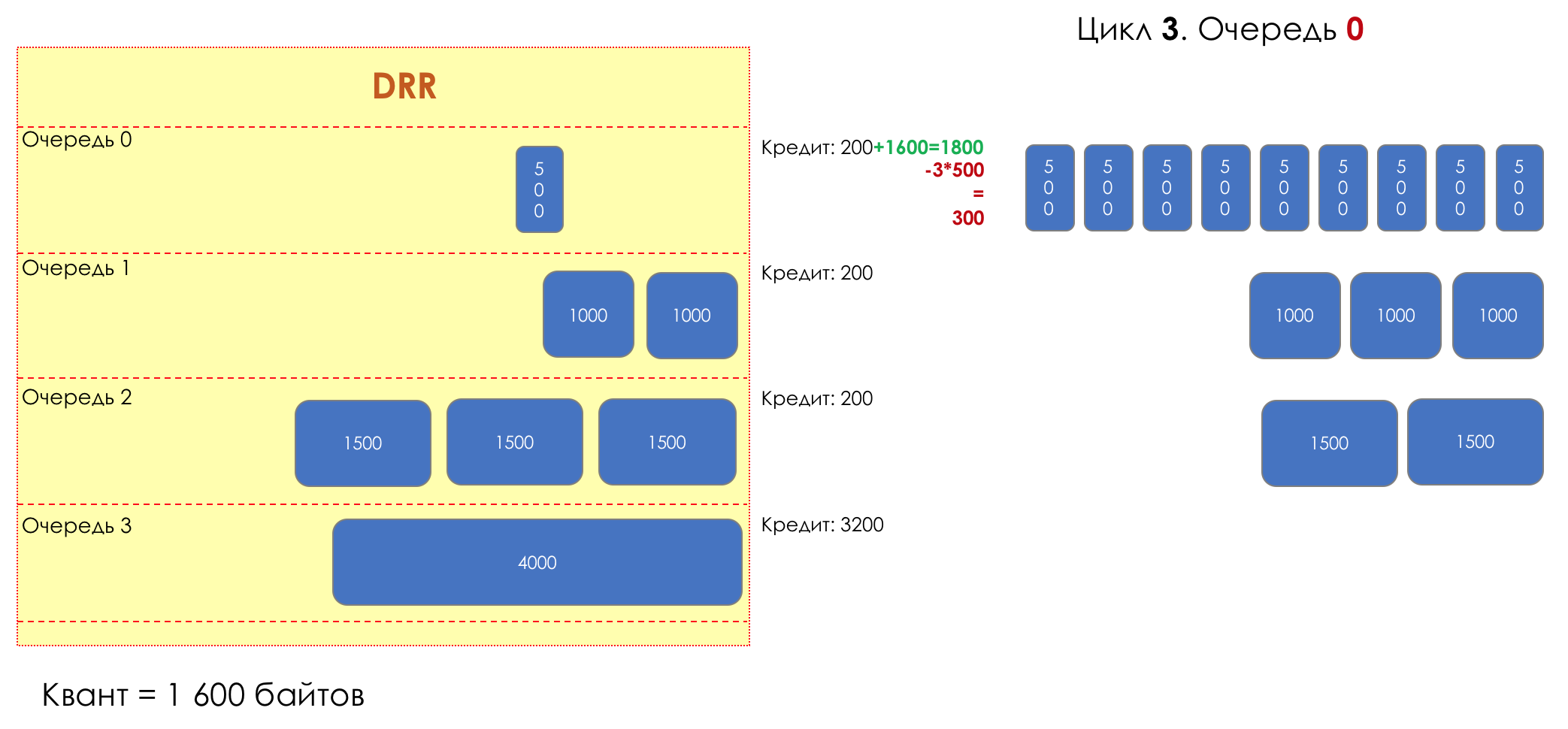
Цикл 3. Очередь 1
Кредит увеличивается до 1800 (200 + 1600).
Один пакет проходит — пропускаем (1800 — 1000 = 800).
Финальный кредит — 800 байтов.
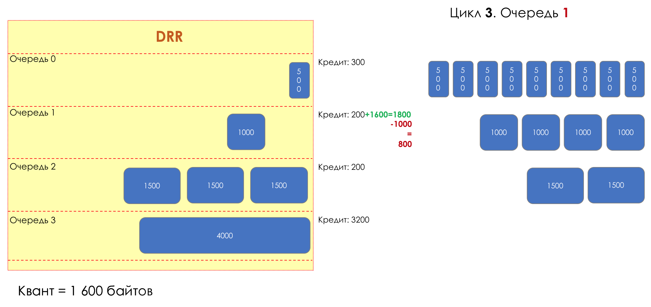
Цикл 3. Очередь 2
Кредит увеличивается до 1800 (200 + 1600).
Один пакет проходит — пропускаем (1800 — 1500 = 300).
Финальный кредит — 300 байтов.

Цикл 3. Очередь 3
Будет и в 3-й очереди праздник!
Кредит увеличивается до 4800 (3200 + 1600).
Пакет наконец проходит — пропускаем (4800 — 4000 = 800).
Финальный кредит — 800 байтов.
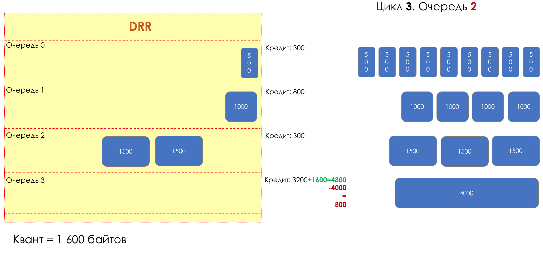
Итак, по окончании третьего цикла работы диспетчера пропустили:
Имеющийся кредит:
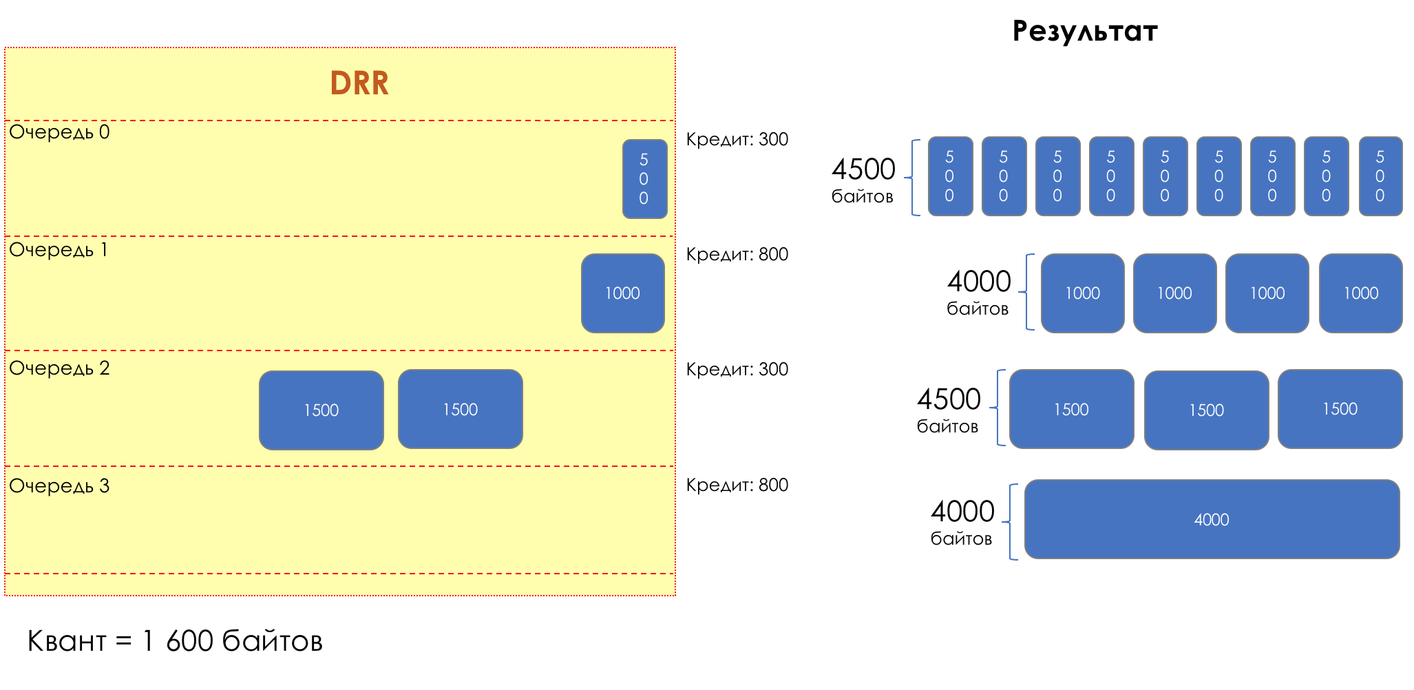
Достаточно наглядна здесь работа DRR. В масштабах многих итераций все очереди получат причитающуюся часть полосы.
Если кому не лень, смотрите анимации.
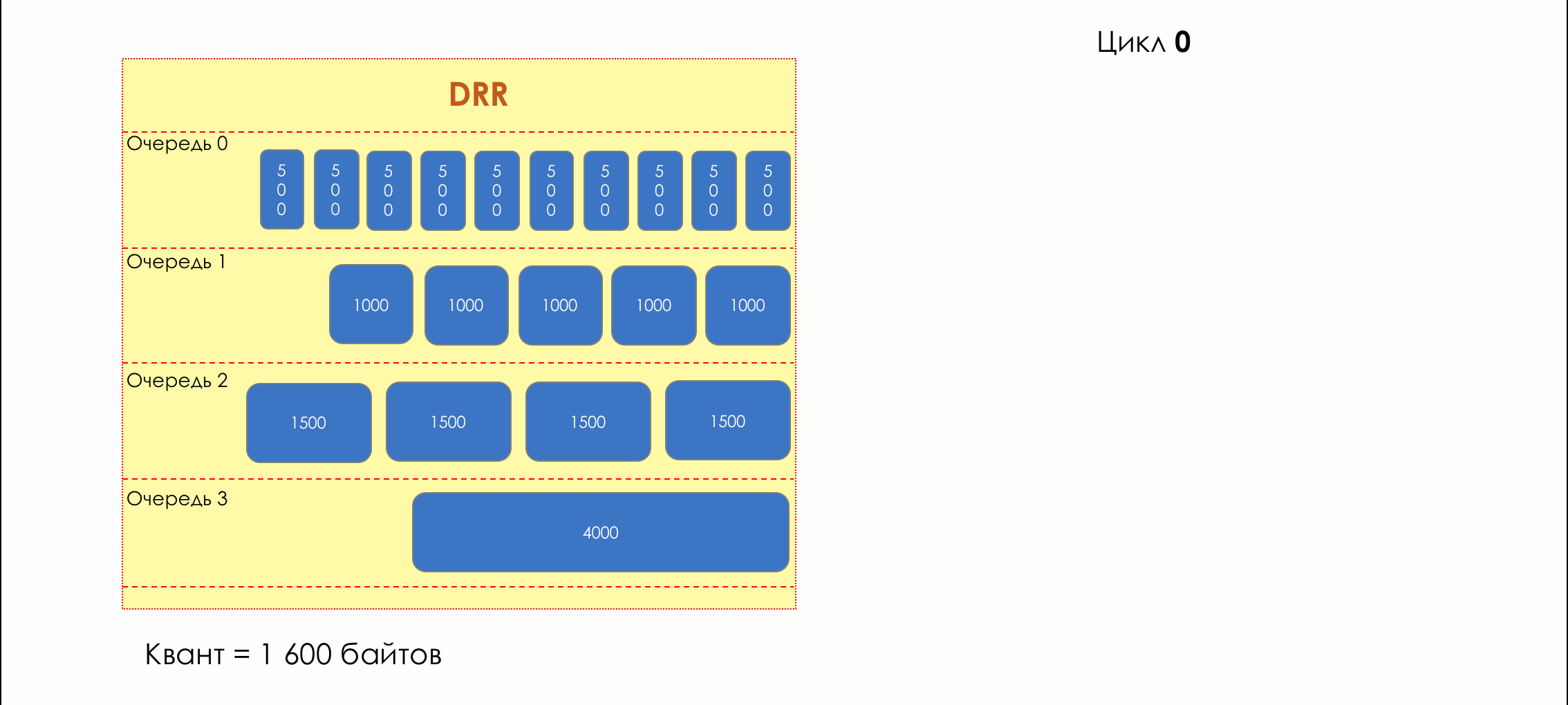
Отличие DWRR от DRR только в том, что в начале цикла каждой очереди выделяется квант, полагающийся именно ей, а не одинаковый для всех.
Выше был описан подход DRR, в котором очереди нельзя уходить в минус — если кредитов не хватает, пакет не пропускается.
Однако есть и более либеральный: пакеты пропускаются, пока очередь не в минусе. В следующий раз пакет пройдёт как только кредит окажется опять положительным.
- DRR (без W),
- 4 очереди,
- в 0-й все пакеты по 500 байтов,
- В 1-й — по 1000,
- Во 2-й по 1500,
- А в 3-й лежит одна колбаса на 4000,
- Квант — 1600 байтов.
Цикл 1
Цикл 1. Очередь 0
Начинается первый цикл, каждой очереди выделяется по 1600 байтов (квант)
Обработка начинается с 0-й очереди. Диспетчер считает:
Первый пакет в очереди проходит — Пропускаем (1600 — 500 = 1100).
Второй — проходит — пропускаем (1100 — 500 = 600).
Третий — проходит — пропускаем (600 — 500 = 100).
Четвёртый — уже не проходит (100 — 500 = -400). Переходим к следующей очереди.
Финальный кредит — 100 байтов.
Цикл 1. Очередь 1
Первый пакет проходит — пропускаем (1600 — 1000 = 600).
Второй не проходит (600 — 1000 = -400). Переходим к следующей очереди.
Финальный кредит — 600 байтов.
Цикл 1. Очередь 2
Первый пакет проходит — пропускаем (1600 — 1500 = 100).
Второй не проходит (100 — 1000 = -900). Переходим к следующей очереди.
Финальный кредит — 100 байтов.
Цикл 1. Очередь 3
Первый пакет уже не проходит. (1600 — 4000 = -2400).
Переходим к следующей очереди.
Финальный кредит — те же 1600 байтов.
Итак, по окончании первого цикла работы диспетчера пропустили:
- Очередь 0 — 1500
- Очередь 1 — 1000
- Очередь 2 — 1500
- Очередь 3 — 0
Имеющийся кредит:
- Очередь 0 — 100
- Очередь 1 — 600
- Очередь 2 — 100
- Очередь 3 — 1600
Цикл 2
В начале цикла к кредиту очереди прибавляется заданный квант — то есть 1600 байтов.
Цикл 2. Очередь 0
Кредит увеличивается до 1700 (100 + 1600).
Первые три пакета в очереди проходят — пропускаем их (1700 — 3*500 = 200).
Четвёртому уже не хватает кредита.
Финальный кредит — 200 байтов.
Цикл 2. Очередь 1
Кредит увеличивается до 2200 (600 + 1600).
Первые два пакета в очереди проходят — пропускаем их (2200 — 2*1000 = 200).
Третий уже не проходит.
Финальный кредит — 200 байтов.
Цикл 2. Очередь 2
Кредит увеличивается до 1700 (100 + 1600).
Первый пакет в очереди проходит — пропускаем его (2200 — 1500 = 200).
А второй — уже нет.
Финальный кредит — 200 байтов.
Цикл 2. Очередь 3
Кредит увеличивается до 3200 (1600 + 1600).
Но она всё равно в пролёте (3200 — 4000 = -800)
Финальный кредит — 3200 байтов.
Итак, по окончании второго цикла работы диспетчера пропустили:
- Очередь 0 — 3000
- Очередь 1 — 3000
- Очередь 2 — 3000
- Очередь 3 — 0
Имеющийся кредит:
- Очередь 0 — 200
- Очередь 1 — 200
- Очередь 2 — 200
- Очередь 3 — 3200
Цикл 3
В начале каждого цикла к кредиту очереди прибавляется квант — 1600 байтов.
Цикл 3. Очередь 0
Кредит увеличивается до 1800 (200 + 1600).
И снова три пакета в очереди проходят — пропускаем их (1800 — 3*500 = 300).
Четвёртому опять не хватает кредита.
Финальный кредит — 300 байтов.
Цикл 3. Очередь 1
Кредит увеличивается до 1800 (200 + 1600).
Один пакет проходит — пропускаем (1800 — 1000 = 800).
Финальный кредит — 800 байтов.
Цикл 3. Очередь 2
Кредит увеличивается до 1800 (200 + 1600).
Один пакет проходит — пропускаем (1800 — 1500 = 300).
Финальный кредит — 300 байтов.
Цикл 3. Очередь 3
Будет и в 3-й очереди праздник!
Кредит увеличивается до 4800 (3200 + 1600).
Пакет наконец проходит — пропускаем (4800 — 4000 = 800).
Финальный кредит — 800 байтов.
Итак, по окончании третьего цикла работы диспетчера пропустили:
- Очередь 0 — 4500
- Очередь 1 — 4000
- Очередь 2 — 4500
- Очередь 3 — 4000
Имеющийся кредит:
- Очередь 0 — 300
- Очередь 1 — 800
- Очередь 2 — 300
- Очередь 3 — 800
Достаточно наглядна здесь работа DRR. В масштабах многих итераций все очереди получат причитающуюся часть полосы.
Если кому не лень, смотрите анимации.
Отличие DWRR от DRR только в том, что в начале цикла каждой очереди выделяется квант, полагающийся именно ей, а не одинаковый для всех.
Выше был описан подход DRR, в котором очереди нельзя уходить в минус — если кредитов не хватает, пакет не пропускается.
Однако есть и более либеральный: пакеты пропускаются, пока очередь не в минусе. В следующий раз пакет пройдёт как только кредит окажется опять положительным.
With the DWRR, the question still remains with the guarantee of delays and jitter - its weight does not solve it at all.
Theoretically, here you can do as with CB-WFQ, adding LLQ.
However, this is just one of the possible scenarios for the popularity of today.
PB-DWRR - Priority-Based DWRR
Actually, PB-DWRR - Priority Based Deficit Weighted Round Robin is becoming almost mainstream today.
This is the same old evil DWRR, to which one more queue has been added - a priority queue, in which packets are processed with a higher priority. This does not mean that it is given a larger band, but the fact that packages will be taken from there more often.
There are several approaches to implementing PB-DWRR. In some of them, as in PQ, any packet arriving at the priority queue is immediately withdrawn. In others, it is accessed every time a controller moves between queues. Thirdly, a credit and a quantum are introduced for it, so that the priority queue could not squeeze the entire strip.
Of course, we will not analyze them.
Short summary about dispatch mechanisms
For decades, mankind has tried to solve the most difficult problem of providing the necessary level of service and fair distribution of the strip. The main tool was queues, the only question was how to pick up packets from the queues, trying to push them into one interface.
Starting with the FIFO, it invented the PQ - the voice was able to coexist with surfing, but there was no speech about the guarantee of the band.
There were several monstrous FQ, WFQ, which worked, if not per-flow, then almost like that. CB-WFQ came to a class society, but did not make it any easier.
As an alternative to him, RR developed. It turned into a WRR, and then a DWRR.
And in the depths of each dispatcher lives FIFO.
However, as you can see, there is not some kind of universal dispatcher, which handled all classes as they require. This is always a combination of controllers, one of which solves the problem of providing delays, jitter and no loss, and the other band allocation.
CBWFQ + LLQ or PB-WDRR or WDRR + PQ.
On real equipment, you can specify which queues to process by which dispatcher.
CBWFQ, WDRR and their derivatives are today's favorites.
PQ, FQ, WFQ, RR, WRR - we do not grieve or remember (unless, of course, we are preparing for the CCIE Clipper).
So, dispatchers are able to guarantee speed, but how to limit it from above?
8. Speed Limit
The need to limit the speed of traffic at first glance is obvious - do not let the client out of the limits of his band according to the contract.
Yes. But not only. Suppose there is a 620 Mb / s RRL span connected via a 1Gb / s port. If the whole gigabit is shot at him, then somewhere on the RRL, which, quite likely, has no idea about queues and QoS, monstrous drops of a random nature will start, not tied to the real priorities of the traffic.
However, if you enable shaping up to 600 Mb / s on the router, then EF, CS6, CS7 will not be discarded at all, and in the BE, AFx, the band and the drops will be distributed according to their weights. Up to RRL will reach 600 MB / s and we will get a predictable picture.
Another example is the admission control. For example, two operators have agreed to trust all the markings of each other, except CS7 - if something has come to CS7 - discard. For CS6 and EF - to give a separate queue with a guarantee of delay and no loss.
But, what if the ingenious partner began to pour torrents into these lines? Goodbye telephony. And the protocols will most likely begin to fall apart.
It is logical in this case to agree with the partner about the band. All that fits into the contract - skip. What does not fit - discarded or transferred to another queue - BE, for example. Thus we protect our network and our services.
There are two fundamentally different approaches to speed limiting: polishing and shaping. They solve one problem, but in different ways.
Consider the difference on the example of such a traffic profile:
Traffic policing
Polising limits the speed by dropping excess traffic.
Anything that exceeds the set value, policer cuts and throws.
What is cut is forgotten. The picture shows that the red packet is not in traffic after the polisher.
And this is how the selected profile will look like after the polisher:
Because of the rigor of the measures taken, this is called Hard Policing .
However, there are other possible actions.
Polyser usually works in conjunction with a traffic meter. The meter paints packages, as you remember, in green, yellow or red.
And on the basis of this color, the policer may not discard the package, but place it in another class. These are soft measures - Soft Policing .
It can be applied to both incoming traffic and outgoing traffic.
A distinctive feature of a polisher is its ability to absorb traffic spikes and determine the peak allowable speed due to the Token Bucket mechanism.
That is, in fact, everything that is above a given value is not cut off - it is allowed to go a little beyond it - short-term bursts or small excesses of the selected band are skipped.
The name “Policing” is dictated by a rather strict attitude of the tool to excess traffic - dropping or de-lowering to a lower class.
Traffic shaping
Shaping limits speed by buffering excess traffic.
All incoming traffic passes through the buffer. A shaper removes packets from this buffer at a constant rate.
If the speed of packet arrival to the buffer is below the output, they do not linger in the buffer - they fly through.
And if the rate of receipt is higher than the output, they begin to accumulate.
The output speed is always the same.
Thus, bursts of traffic are buffered and will be sent when it comes to their turn.
Therefore, along with scheduling in queues, shaping is the second tool contributing to the aggregate latency .
The illustration clearly shows how a packet arriving at the time t2 buffer appears at the output at time t3. t3-t2 is the delay introduced by the shaper.
Shaper is usually applied to outgoing traffic.
This is the profile after the shaper.
The name “Shaping” indicates that the tool gives shape to the traffic profile, smoothing it out.
The main advantage of this approach is the optimal use of the available band - instead of dropping excessive traffic, we postpone it.
The main drawback - the unpredictable delay - when filling the buffer, the packets will languish in it for a long time. Therefore, shaping is not suitable for all types of traffic.
Shaping uses the Leaky Bucket mechanism.
Shaping against polising
The work of a polisher is similar to a knife, which, moving along the surface of the oil, cuts off the sharp side of the tubercle.
The work of the shaper is like a roller, which smoothes the tubercles, distributing them evenly over the surface.
Shaper tries not to drop packets while they are being buffered at the cost of increasing latency.
Polysser does not introduce delays, but more readily discards packets.
Applications that are not sensitive to delays, but for which losses are undesirable, should be limited to a shaper.
For those for whom a late packet is like a lost one, it is better to drop it immediately - then polysing.
Shaper does not affect packet headers or their fate outside the node, while after polishing, the device can remake the class in the header. For example, the packet had an AF11 class at the entrance, the metering colored it yellow inside the device, it remarked its class at AF12 at the exit — on the next node it will have a higher drop probability.
Practice polising and shaping
The scheme is the same:
Configuration file. We
see this picture without applying restrictions:
We will proceed as follows:
- On the input interface Linkmeup_R2 (e0 / 1) we configure polishing - this will be the input control. Under the contract, we give 10 MB / s.
- On the output interface Linkmeup_R4 (e0 / 2) we configure the shaping to 20 Mb / s.
Let's start with the shaper on Linkmeup_R4 .
Match all:
class-map match-all TRISOLARANS_ALL_CM
     match any
Shape to 20Mb / s:
policy-mapTRISOLARANS_SHAPINGclassTRISOLARANS_ALL_CMshapeaverage 20000000Apply to the output interface:
interfaceEthernet0/2
     service-policy output TRISOLARANS_SHAPING
All that must leave (output) interface Ethernet0 / 2, shape up to 20 Mb / s.
Shaper configuration file.
And here is the result:
A fairly smooth line of total throughput and ragged graphics for each individual stream is obtained.
The fact is that we limit the overall lane with the shaper. However, depending on the platform, individual streams can also be individually shaped, thus obtaining equal opportunities.
Now let's set up polishing for Linkmeup_R2.
We will add a policer to the existing policy.
policy-map TRISOLARANS_ADMISSION_CONTROL
    class TRISOLARANS_TCP_CM
     police cir 10000000 bc 1875000 conform-action transmit exceed-action drop
The interface policy has already been applied:
    interface Ethernet0/1
     service-policyinput TRISOLARANS_ADMISSION_CONTROL
Here we indicate the average allowed speed of CIR (10Mb / s) and the allowed burst of Bc (1,875,000 bytes about 14.6 MB).
Later, explaining how the polisher works, I will tell you what CIR and Bc are and how to determine these values.
Polyser configuration file.
This picture is observed with polising. Immediately see dramatic changes in the level of speed:
But such a curious picture is obtained if we make the allowable burst size too small, for example, 10,000 bytes.
police cir 10000000 bc 10000 conform-action transmit exceed-action dropThe overall speed immediately dropped to about 2Mb / s.
Be careful with setting up the bursts :)
Test table.
Leaky Bucket and Token Bucket Mechanisms
It sounds easy and understandable. But how does it work in practice and is it implemented in hardware?
Example.
Is the limit of 400 MB / s a lot (or a little)? On average, the client uses only 320. But sometimes it rises to 410 for 5 minutes. And sometimes up to 460 for a minute. And sometimes up to 500 for half a second.
As a contractual provider, linkmeup can say - 400 and that's that! Want more, connect to the tariff 1Gb / s + 27 anime channels.
And we can increase customer loyalty, if it does not interfere with others by allowing such bursts.
How to allow 460Mb / s for just one minute, not 30 or forever?
How to allow 500 MB / s, if the band is free, and press up to 400, if there are other consumers?
Now take a break, pour a strong bucket.
Let's start with a simpler mechanism used by the shaper - a flowing bucket.
Leaky bucket algorithm
Leaky Bucket is a leaking bucket.
We have a bucket with a hole of a given size at the bottom. Packages are poured into this bucket on top. And from the bottom they flow with a constant bit rate.
When the bucket fills, new packages begin to be discarded.
The hole size is determined by the specified speed limit, which for Leaky Bucket is measured in bits per second.
The volume of the bucket, its fullness and output speed determine the delay introduced by the shaper.
For convenience, the bucket volume is usually measured in ms or μs.
In terms of implementation, Leaky Bucket is a regular SD-RAM based buffer.
Even if the shaping is not explicitly configured, in the presence of bursts that do not pass into the interface, the packets are temporarily added to the buffer and transmitted as the interface is released. This is also shaping.
Leaky Bucket is used only for shaping and is not suitable for poliscing.
Algorithm Token Bucket
Many believe that Token Bucket and Leaking Bucket are one and the same. Stronger was only Einstein's fault, adding the cosmological constant.
Switching chips are not very well aware of what time is, they consider even worse how many bits they transmitted per unit of time. Their job is to thresh.
Is this approaching bit another 400,000,000 bits per second, or is it already 400,000,001?
ASIC developers had a non-trivial engineering challenge.
She was divided into two subtasks:
- Actually speed limit by dropping excess packets based on a very simple condition. It is carried out on switching chips.
- Creating this simple condition, which deals with a more complex (more specialized) chip, leading the expense of time.
The algorithm that solves the second problem is called Token Bucket. His idea is elegant and simple (no).
The task of Token Bucket is to allow traffic if it fits within the limit and discard / dye red if not.
At the same time, it is important to allow bursts of traffic, as this is normal.
And if in Leaky Bucket the bursts were absorbed by the buffer, then Token Bucket does not buffer anything.
Single Rate - Two Color Marking
Do not pay attention to the name yet =)
We have a bucket in which coins fall at a constant speed - 400 mega-coins per second, for example.
The volume of the bucket is 600 million coins. That is, it is filled in a half second.
Nearby are two conveyor belts: one brings packages, the second - takes away.
To get on the conveyor belt, the package must pay.
Coins for this he takes from the bucket in accordance with its size. Roughly speaking - how many bits - so many coins.
If the bucket is empty and the package is not enough coins, it is painted in red signal color and discarded. Alas, mudflows. At the same time, coins are not removed from the bucket.
The next package of coins may already be enough - firstly, the package may be smaller, and, secondly, more coins will attack during this time.
If the bucket is already full, all new coins will be thrown away.
It all depends on the rate of arrival of packages and their size.
If it is consistently lower than or equal to 400 MB per second, then there will always be enough coins.
If higher, then some packets will be lost.
A more specific example with gifs, as we all love.Why bucket volume? The bitstream is not always uniform, it is obvious. The 400 MB / s limit is not an asymptote - traffic can cross it. The volume of stored coins allows small bursts to fly by without being discarded, but the average speed is kept at 400Mb / s.
- There is a bucket with a capacity of 2500 bytes. At the initial moment of time there are 550 tokens in it.
On the pipeline, three packets of 1000 bytes, which want to be sent to the interface.
In each time slot, 500 bytes are dropped into the bucket (500 * 8 = 4 000 bits / time quantum - limiting the polisher).- At the end of the first time slot, 500 tokens fall into the bucket. And at this time, the first package is suitable. Its size is 1000 bytes, and in the bucket 1050 tokens - enough . The package is painted in green and skipped. 1000 tokens are removed from the bucket.
There are 50 tokens in the bucket.- At the end of the second time slot, another 500 tokens fall into the bucket - a total of 550. And the size of the incoming packet - 1000 - is not enough .
The package is painted red and discarded, the tokens are not removed.- At the end of the third quantum, another 500 tokens fall into the bucket - again 1050. The size of the incoming packet - 1000 - is enough .
The package is painted in green and skipped, tokens are removed from the bucket.
A bucket of 2500 bytes actually means that a package with more than 2500 bytes will never pass through such a polisher, it will never have enough tokens. Therefore, its volume should not be less than MTU and generally it is recommended that a volume equal to the amount of traffic at the maximum speed allowed by the polisher, in 1.5-2 seconds.
That is, the formula is as follows:
CBS = CIR (bits per second) * 1.5 (seconds) / 8 (bits per byte)
If you go back to the practical example of polysing, where we set up bursts (Bc), it becomes clear that with large value (1 875 000 bytes) all bursts are depreciated well. And with a small one (10,000 bytes), despite the fact that it is noticeably larger than the MTU, the polisher reverts to the constant filling of the bucket and discards a large number of packets.
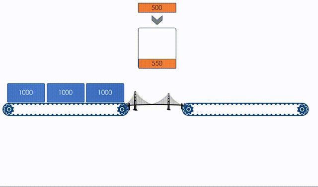
For example, a stable stream of 399 MB / s for 600 seconds will allow the bucket to fill to the brim.
Further, traffic can go up to 1000Mb / s and stay at this level for 1 second - 600 Mm (Megamonet) of the stock and 400 Mm / s of the guaranteed band.
Or the traffic can rise up to 410 Mb / s and stay that way for 60 seconds.
That is, the stock of coins allows you to slightly go beyond the limit for a long time or throw out a short but high burst.
Now to the terminology.
The rate of arrival of coins in a bucket - CIR - Committed Information Part Rate (Guaranteed average speed). Measured in bits per second.
The number of coins that can be stored in a bucket - CBS - Committed Burst Size . Maximum allowed burst size. Measured in bytes. Sometimes, as you may have noticed, is called Bc .
Tc - The number of coins (Token) in the C bucket (CBS) at the moment.
In the article, I use the term " Tc ", just as it is used in RFC 2697 ( A Single Rate Three Color Marker ).This is the easiest scenario. It is called Single Rate - Two Color .
However, there is another Tc, which describes the time interval when a new batch of coins is poured into a bucket.
There should be a retreat.
It is impossible to tune the speed of the interface to satisfy the conditions of a polisher, and therefore the Token Bucket system is introduced, which essentially implements TDM (Time-Division Multiplexing) - it allows sending traffic only at certain points in time.
That is, the coins do not flow into the bucket in a continuous stream - the modern world, alas, is discrete.
As a first approximation, it is proposed to pour CIR coins once per second. Then after a second and so on.
It works badly, because a surge - and a second of silence, a surge - and a second of silence, a surge - and a second of silence.
Therefore, in the second approximation, the second is divided into time intervals, in which a certain number of coins descend.
This time interval is also called (at least in the Cisco literature) Tc , and the number of falling coins is called Bc . In this case, Bc = CIR * Tc .
That is, at the beginning of each Tc interval, Bc coins are lowered into the bucket.
Single Rate means that there is only one average allowed speed, and Two Color - that you can paint traffic in one of two colors: green or red.
- If the number of available coins (bits) in the C bucket is more than the number of bits that you need to skip at the moment, the package is painted green - low probability of discarding later. Coins are withdrawn from the bucket.
- Otherwise, the package is painted in red - a high probability of a drop (or, more often, a momentary drop). Coins thus buckets C is withdrawn .
Used for polysing in PHB CS and EF, where speeding is not expected, but if it happens, it is better to drop it immediately.
Further we will consider more difficult: Single Rate - Three Color.
Single Rate - Three Color Marking
The disadvantage of the previous scheme is that there are only two colors. What if we do not want to discard everything that is above the average allowed speed, but want to be even more loyal?
the TCM-sr ( Single Rate - the Three the Color The Marking ) enters the second bucket in - E . At this time, the coins are not placed in a bucket filled with the C , are poured into E . EBS is
added to CIR and CBS - Excess Burst Size - The allowed burst size during peaks. Te - the number of coins in a bucket E .
Suppose a package of size B came through the pipeline. Then
- If there is enough coins in the C bucket , the bag is painted in green and is skipped. From the bucket C, B coins are removed (Remains: Tc - B).
- If there is not enough coins in bucket C , bucket E is checked . If there are enough coins in it, the package is painted yellow (the average probability of a drop), and B coins are taken out from the bucket E.

- If there is not enough coins in the E bucket , then the bag is painted in red, coins are not removed from anywhere.

Please note that for a specific package Tc and Te are not cumulative .
That is, a packet of 8000 bytes in size will not pass, even if there are 3000 coins in the C bucket and 7000 coins in the E. There is not enough in C , in E there is not enough - we put a red stamp - shurui from here.
This is a very elegant scheme. All traffic that fits into the average CIR + CBS limit (the author knows that it is impossible to directly add bits / s and bytes) - goes green. At peak times when the customer has exhausted the coins in the C bucket , he still has the stock of Te in the E bucket accumulated during the downtime .
That is, you can skip a little more, but in the case of congestion, these are more likely to be discarded.
sr-TCM is described in RFC 2697 .
Used for polysing in PHB AF.
Well, the last system is the most flexible and therefore complex - Two Rate - Three Color.
Two Rate - Three Color Marking
The Tr-TCM model was born from the idea that, not to the detriment of other users and types of traffic, why shouldn't the client be given a bit more pleasant opportunities, and even better to sell.
Let's tell him that he is guaranteed 400 Mb / s, and if there are free resources, then 500. Are you ready to pay 30 rubles more?
Added another bucket P .
Thus:
CIR - guaranteed average speed.
CBS is the same allowed burst size (bucket volume C ).
PIR - Peak Information Rate - the maximum average speed.
EBS is the allowed burst size during peaks (Bucket Volume P ).
Unlike sr-TCM, tr-TCM now in both buckets are independently received coins. In C - with CIR speed, in P - PIR.
Which rules?
A b- byte packet arrives .
- If there are not enough coins in the P bucket , the bag is marked in red. Coins can not be removed . Otherwise:
- If there is not enough coins in the C bucket , the package is marked yellow, and B coins are removed from the P bucket . Otherwise:
- The package is marked green and B coins are removed from both buckets .
That is, the rules in tr-TCM are different.
As long as traffic keeps within guaranteed speed, coins are taken out of both buckets. Due to this, when the coins run out in the C bucket , they will remain in P , but just enough to not exceed the PIR (if it were taken out only from C , then P would fill more and give a much higher speed).
Accordingly, if it is higher than guaranteed, but lower than the peak, coins are removed only from P , because there is already nothing in C.
tr-TCM monitors not only bursts, but also constant peak speed.
tr-TCM is described in RFC 2698 .
Also used for polysing in PHB AF.
Speed Summary Summary
While shaping puts off traffic when it is exceeded, polishing discards it.
Shaping is not suitable for applications that are sensitive to delays and jitter.
To implement polishing in hardware, the algorithm is Token Bucket, for shaping - Leaky Bucket.
Token Bucket can be:
- With one bucket - Single Rate - Two Color Marking. Allows acceptable bursts.
- With two buckets - Single Rate - Three Color Marking (sr-TCM). Surplus from the C bucket (CBS) is poured into the bucket E. Allows acceptable and surplus bursts.
- With two buckets - Two Rate - Three Color Marking (tr-TCM). Buckets C and P (PBS) are replenished independently at different speeds. Allows peak speed and allowable and excess bursts.
sr-TCM focuses on traffic over limit. tr-TCM - at the rate at which it arrives.
Polising can be used on the input and output from the device. Shaping mainly at the exit.
For PHB CS and EF, Single Rate Two Color Marking is used.
For AF, sr-TCM or tr-TCM.
For perhaps a better understanding, I recommend turning to the original RFC or reading here .
The mechanism of Token Bucket is quite applicable in everyday life. For example, if I go with friends to a bar, while my wife spends time with two children, then every minute a token is taken out of the bucket.
If I draw all the buckets, I can't go for a run over the weekend - I wait while I drift. If there are few tokens, then you can run for an hour, but to go to work on weekends to get involved in an article - no longer.
True bucket filling rate is not constant, tokens stand out for good deeds. In fact, here is a system of two connected buckets - mine and my wife. But you can write to the whole article as well.
Above, I described all the basic QoS mechanisms, if not to go into hierarchical QoS. The most complex system with numerous moving parts.
Everything is good (right?) It has sounded so far, but what is happening under the vanilla outer panel of the router?
Over the years, vendors added more and more konutry, developed sophisticated chips, expanded buffers to keep pace with the growing volume of traffic and its new categories, on the one hand, and to solve the growing problems caused by the first item, on the other.
Continuing race. You can not lose packages if a competitor does not lose them. You can not abandon the functionality if the opponent is with him under the doors of the customer.
Ida in the lair of proprietary!
9. Hardware QoS implementation
In this chapter, I take on the ungrateful task. If you describe as simple as possible, there will always be those who say that everything is not so in reality.
If you describe it as it is, the reader will drop the article, because it will turn into a drawing of a submarine, more precisely the drawings of three boats with pencils of different colors on one sheet.
In general, I will make a disclaimer that in reality everything is not as it really is, and will follow the simple version.
Forgive me, my companion perfectionist.
What controls the behavior of the node and starts the appropriate mechanisms in relation to the package? The priority that he carries in one of the headers? Yes and no.
As mentioned above, a standard switching header usually ceases to exist within a network device.
As soon as the packet has got on the switching chip, the headers are removed from it and sent for analysis, and the payload is languishing in some kind of temporary buffer.
Based on the headers, a classification occurs (BA or MF) and the decision to transfer is made.
In an instant, an internal header with package metadata is attached to the packet.
This metadata carries a lot of important information - the sender and recipient addresses, the output chip, the cell sequence number, if there was packet fragmentation and necessarily class marking (CoS) and drop priority (Drop Precedence). Only marking in the internal format - it may or may not coincide with the DSCP.
In principle, inside the box you can set an arbitrary length of the marking, not being tied to the standards, and determine very flexible actions with the package.
At Cisco, the internal labeling is called QoS Group, at Juniper - Forwarding Class, Huawei has not decided: it calls internal priorities, somewhere local priorities, Service-Class somewhere, and CoS somewhere. Add in comments names for other vendors - I will add.
This internal marking is assigned based on the classification that the node has performed.
It is important that if not stated otherwise, the internal marking only works inside the node, but then it doesn’t appear on the label in the headers of the packet that will be sent from the node - it will remain the same.
However, at the entrance to the DS-domain after classification, a remarking into a certain class of service adopted in this network usually occurs. Then the internal marking is converted to the value adopted for this class on the network, and is written in the header of the packet being sent.
The internal marking of CoS and Drop Precedence only defines the behavior inside this node and is not explicitly passed on to its neighbors, except for remarking the headers.
CoS and Drop Precedence determine the PHB, its mechanisms and parameters: overload prevention, congestion management, dispatching, remarking.
Through what circles pass the packets between the input and output interfaces I discussed in the previous article . Actually, it turned out to be unplanned, since at some point it became obvious that it was premature to talk about QoS without an understanding of the architecture.
However, let's repeat.
- The signal goes to the physical input interface and its chip (PIC). A bitstream flows from it and then a packet with all the headers.
- Next to the input switching chip (FE), where the headers are separated from the packet body. There is a classification and it is determined where the package should be sent further.
- Next to the input queue (TM / VOQ). Already here, packages are laid out in different queues based on their class.
- Next to the switching factory (if there is one).
- Next to the output queue (TM).
- Next to the output switching chip (FE), where new headers are hung.
- Next to the output interface (possibly through another queue) (PIC).
In this case, the router must solve a complex equation.
Spread out all the classes, provide someone with a wide band, someone low latency, someone to ensure the absence of losses.
And at the same time have time to skip all traffic if possible.
In addition, you need to do shaping, possibly polishing. If suddenly there is an overload, then cope with it.
And that's not counting Lukap, processing ACL, statistics calculation.
Unenviable share. But robots are driving, not man.
In fact, there are only two places where the QoS mechanisms work - the switching chip and the traffic management / queue chip.
At the same time on the switching chip, operations occur that require analysis or actions with headers.
- Classification
- Polising
- Remarking
The rest is taken by TM. These are mainly routine operations with a predefined algorithm and adjustable parameters:
- Overload prevention
- Congestion management
- Shaping
TM is a smart buffer, usually based on SD-RAM.
He is smart because, a) programmable, b) with queues he knows how to do all sorts of tricky things.
It is often distributed — SD-RAM chips are located on each interface board, and together they combine into a VOQ (Virtual Output Queue) that solves the problem Head of Line Blocking.
The fact is that if the switching chip or the output interface is flooded, then they ask the input chip to slow down and not send traffic for some time. If there is only one queue in all directions, then it is very disappointing that all the others suffer from one output interface. This is the Head of Line Blocking.
VOQ creates multiple virtual output queues for each existing output interface on the input interface board.
Moreover, these lines in modern equipment take into account the labeling of the package.
About VOQ described in sufficient detail in a series of notes here .
By the way, the lines are actually placed, they are promoted, not the packages themselves, but only the records about them, are being withdrawn, etc. It makes no sense to do so many gestures with large arrays of bits. While QoS is being measured over the records, the packets are fine in the memory and retrieved from there to the address.
VOQ is a software queue (the English term Software Queue is more accurate). After it, immediately before the interface there is also a hardware queue, which always, strictly works on FIFO. It’s almost impossible to control any of its parameters (for example, Cisco allows you to adjust only the depth using the tx-ring-limit command).
Just between the software and hardware queue, you can run arbitrary dispatchers. It is in the program queue that Head / Tail-drop and AQM, polishing and shaping work.
The size of the hardware queue is very small (units of packages), because the dispatcher does all the work of placing in the line-rate.
Unfortunately, you can make a lot of reservations here, and in general, cross out everything with a red pen and say “it’s not like that with vendor X”.
I would like to make one more remark about service packages. They are handled differently than transit user packets.
Being generated locally, they are not checked for compliance with ACL rules and speed limits.
The packets from the outside, destined for the CPU, from the output switching chip fall into other queues — to the CPU — based on the protocol type.
For example, BFD has the highest priority, OSPF can wait a little longer, and ICMP and generally not afraid to drop. That is, the more important the packet is for network performance, the higher its class of service is when sending to the CPU. That is why seeing in ping or tracing varying delays on transit hops is normal - ICMP is not a priority for CPU traffic.
In addition, protocol packets applyCoPP - Control Plane Protection (or Policing) - speed limits to avoid high CPU utilization - again, better predictable drops in low priority queues before problems start.
CoPP will help from both targeted DoS and abnormal network behavior (for example, loops) when a lot of broadcast traffic begins to arrive on the device.
useful links
- The best book on the theory and philosophy of QoS: QOS-Enabled Networks: Tools and Foundations .
Some excerpts from it can be read here , but I would recommend reading it in and out without exchanging it. - Surprisingly detailed and well written book about QoS from Huawei: Special Edition QoS (v6.0) . The equipment architecture and PHB work on different boards are very well versed.
- A very detailed comparison of sr-TCM and tr-TCM from Aini: Understanding Single-Rate and Dual-Rate Traffic Policing .
- About VOQ: What is VOQ and why should you care?
- About QoS in MPLS: MPLS and Quality of Service .
- A relatively brief QoS brief on the example of Juniper: Juniper CoS notes .
- Virtually all QoS is one way or another focused on the specifics of TCP and UDP. It would not be superfluous to thoroughly understand them: The TCP / IP Guide
- Well, for those who do not feel in themselves the strength to overcome all this work, the Shaggy Mammoth wrote a separate note for you: Looking for a lost gigabit or a bit about windows in TCP .
- This page is difficult, but it describes in detail how the mechanisms of the FQ: Queuing and Scheduling group work .
And if you go up a level, a large-scale open document will open, called An Introduction to Computer Networks , injecting paint, because the Introduction is so powerful that I don’t know half there. Even the most wanted to read. - About WFQ is very scientific, but with intelligence that I obviously don’t have, it’s also clear in colors: Weighted Fair Queueing: a packetized approximation for FFS / GP.
- There is also the LFI mechanism, which I didn’t touch upon, because it is not very important in our realities to have a stigabyte interface, but it may be interesting to get acquainted: Link Fragmentation and Interleaving .
And, of course, the RFC set ...
- tools.ietf.org/html/rfc791 (INTERNET PROTOCOL)
- tools.ietf.org/html/rfc1349 (Type of Service in the Internet Protocol Suite)
- tools.ietf.org/html/rfc1633 (Integrated Services in the Internet Architecture: an Overview)
- tools.ietf.org/html/rfc2474 (Definition of the Differentiated Services Field (DS Field) in the IPv4 and IPv6 Headers)
- tools.ietf.org/html/rfc2475 (An Architecture for Differentiated Services)
- tools.ietf.org/html/rfc2597 (Assured Forwarding PHB Group)
- tools.ietf.org/html/rfc2697 (A Single Rate Three Color Marker)
- tools.ietf.org/html/rfc2698 (A Two Rate Three Color Marker)
- tools.ietf.org/html/rfc3031 (Multiprotocol Label Switching Architecture)
- tools.ietf.org/html/rfc3168 (The Addition of Explicit Congestion Notification (ECN) to IP)
- tools.ietf.org/html/rfc3246 (An Expedited Forwarding PHB (Per-Hop Behavior))
- tools.ietf.org/html/rfc3260 (New Terminology and Clarifications for Diffserv)
- tools.ietf.org/html/rfc3662 (A Lower Effort Per-Domain Behavior (PDB) for Differentiated Services)
- tools.ietf.org/html/rfc4594 (Configuration Guidelines for DiffServ Service Classes)
- tools.ietf.org/html/rfc5462 (Multiprotocol Label Switching (MPLS) Label Stack Entry: «EXP» Field Renamed to «Traffic Class» Field)
Conclusion
This release has had many reviewers.
Thank.
Alexander Fatinu ( LoxmatiyMamont ) for introductory words and valuable tips on the expressiveness and clarity of the text.
Alexander Clipper (@ metallicat20) for peer review.
Alexandru Klimenko (@ v00lk) for harsh criticism and the most massive changes in recent days.
Andrei Glazkov (@glazgoo) for comments on structure, terminology and commas.
Artem Chernobay for KDPV.
Anton Klochkov (@NAT_GTX) for contacts with Miran.
Miran (miran.ru) for organizing a server with Eve and broadcast. Traditionally, my family, which, incidentally, this time suffered the least because of her absence next to the most difficult moments.