Richard Hamming: Chapter 20. Modeling - III

“The goal of this course is to prepare you for your technical future.”

It remains to publish 2 chapters ...

Modeling - III

I will continue the general direction given in the previous chapter, but this time I will concentrate on the old expression “Garbage at the entrance - garbage at the exit”, which is often abbreviated as GIGO (garbage in, garbage out). The idea is that if you put inaccurately collected data and incorrectly defined expressions on an input, then you can only get incorrect results on the output. The opposite is also implicitly assumed: from the availability of accurate input data, it follows that a correct result is obtained. I will show that both of these assumptions can be false.

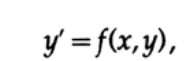
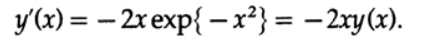
Often, the simulation is based on solving differential equations, so first we consider the simplest first-order differential equation of the form



As you remember, the field of directions is the lines constructed at each point of the xy plane, with the angular coefficients given by the differential equation (Figure 20.I). For example, a differential equation has a direction field, shown in Figure 20.II.





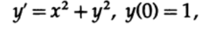
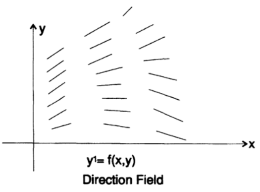
Figure 20.I

For each concentric circle,



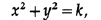
such that the slope of the straight line is always the same and depends on the value of k. Such curves are called isoclines .

And now we will look at the field of directions of another differential equation (Figure 20.III). In the left part, we see a divergent field of directions, which means that small changes in the initial values ​​or small computation errors will lead to a large difference in the values ​​in the middle of the trajectory. In the right part we see that the field of directions converges. This means that with a larger difference of values ​​in the middle of the trajectory, the difference in values ​​at the right end will be small. This simple example shows how small errors can become large, large errors small, and moreover, how small errors can first become large and then small again. Therefore, the accuracy of the solution depends on the specific interval on which the solution is calculated. There is no absolute general accuracy.



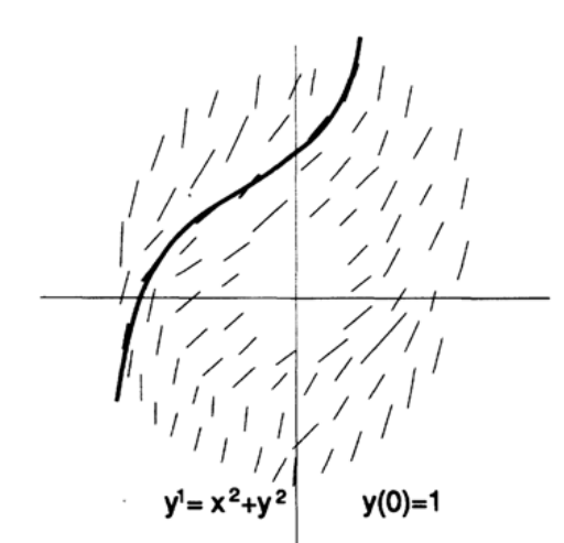
Figure 20.II



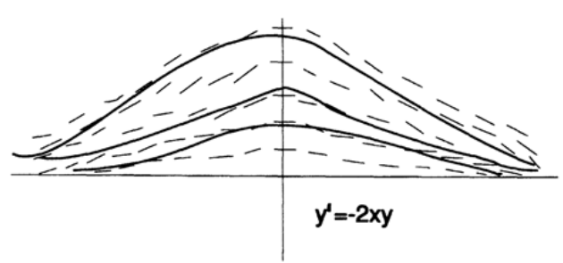
Figure 20.III

These arguments are built for the function


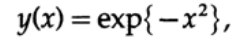
which is a solution to a differential equation



Probably, you have already presented a "pipe", which first expands and then narrows around the "true, exact solution" of the equation. This representation is excellent for the case of two dimensions, but when I have a system of n such differential equations — 28 in the case of the interceptor missile problem for the Navy mentioned earlier — then these “pipes” around the true solution of the equation turn out to be nothing at first sight. A figure consisting of four circles in two dimensions leads to the n-dimension paradox described in Chapter 9 for ten-dimensional space. This is just another look at the problem of stable and unstable modeling described in the previous chapter. This time I will give specific examples related to differential equations.

How do we solve differential equations numerically? Starting from the usual differential equation of the first order, we represent the field of directions. Our task is to have a given initial value to calculate the value at the next nearest point of interest. If we take the local coefficient of the slope of the line, given by the differential equation, and take a small step forward tangentially, we will introduce only a small error (Figure 20.IV).

Using this new point we will move to the next point, but as you can see in the figure, we gradually deviate from the true curve, because we use the slope coefficient of the previous step, rather than the true slope coefficient for the current interval. To avoid this effect, we “predict” some value, then use it to estimate the angular coefficient at this point (using the differential equation), and then use the average value of the angular coefficient at the two interval boundaries as the angular coefficient for this interval.

Then, using this averaged angular coefficient, we take another step forward, this time using the “correction” formula. If the values ​​obtained using the “prediction” and “correction” formulas are close enough, then we assume that our calculations are accurate enough, otherwise we must reduce the step size. If the difference between the values ​​is too small, then we must increase the step size. Thus, the traditional “predictor-corrector” scheme has a built-in mechanism for checking the error at each step, but this error at a particular step is in no way and in any sense a common accumulated error! It is absolutely clear that the accumulated error depends on whether the field of directions converges or diverges.



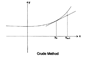
Figure 20.IV



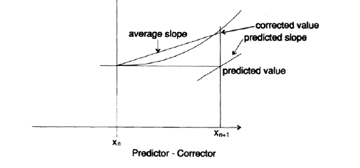
Figure 20.V

We used simple straight lines for both the prediction step and the correction step. The use of polynomials of higher degrees gives a more accurate result; Quarter-degree polynomials are usually used (the solution of differential equations by the Adams – Bashfort method, the Milne method, the Hamming method, etc.). Thus, we have to use the values ​​of the function and its derivatives at several previous points to predict the value of the function at the next point, after which we use the substitution of this value into the differential equation and approximate the new value of the slope. Using the new and previous values ​​of the angular coefficient as well as the values ​​of the desired function, we adjust the resulting value. It's time to notice that the corrector is nothing more than a digital recursive filter,

Stability and other concepts discussed earlier remain relevant. As mentioned earlier, there is an additional feedback loop for the predicted solution of a differential equation, which in turn is used in the calculation of the corrected slope. Both of these values ​​are used in solving a differential equation, recursive digital filters are just formulas, and nothing more. However, they are not the transfer characteristics, as they are commonly considered in the theory of digital filters. In this case, the values ​​of the differential equation are simply calculated. At the same time, the difference between the approaches is significant: in digital filters linear signal processing takes place, while in solving differential equations there is nonlinearity, which is introduced by calculating the values ​​of the derived functions. This is not the same as a digital filter.

If you solve a system of n differential equations, then you are dealing with a vector of n components. You predict the next value of each component, evaluate each of the n derivatives, correct each of the predicted values, and then accept the result of the calculations at this step or reject it if the local error is too large. You tend to think of small errors as a “tube” surrounding a true calculated path. And I call again to remember the paradox of the four circles, in high-dimensional spaces. Such "pipes" may not be what they seem at first glance.

Now let me point out the significant difference between the two approaches: computational methods and the theory of digital filters. In common textbooks, only computational mathematics methods are described that approximate functions by polynomials. Recursive filters use frequencies in evaluation formulas! This leads to significant differences!

To see the difference, let's imagine that we are developing a simulator for landing a man on Mars. The classical approach concentrates on the shape of the landing trajectory and uses approximation by polynomials for local regions. The resulting path will have break points in acceleration, as we move step by step from interval to interval. In the case of the frequency approach, we will focus on getting the correct frequencies and let the location be what it is. In the ideal case, both trajectories will be the same, in practice they may differ significantly.

Which campaign should I use? The more you think about it, the more you will be inclined to think that the pilot in the simulator wants to get a “feeling” of the behavior of the boarding module, and it seems that the frequency response of the simulator should be well “felt” by the pilot. If the location is slightly different, the feedback loop will compensate for this deviation in the landing process, but if the control “feel” is different during a real flight, the pilot will be concerned about new “sensations” that were not in the simulator. It always seemed to me that simulators should prepare pilots for real sensations as much as possible (of course, we cannot imitate reduced gravity on Mars for a long time) in order for them to feel comfortable when in reality they face a situation with which they repeatedly encountered in the simulator. Alas, we know too little about what the pilot "feels." Does the pilot sense only real frequencies from the Fourier expansion, or do they also sense the complex damped frequencies of Laplace (or maybe we should use wavelets?). Do different pilots feel the same things? We need to know more than we know now about these essential design conditions.

The situation described above is a standard contradiction between the mathematical and engineering approach to solving a problem. These approaches have different goals in solving differential equations (as in the case of many other problems), therefore they lead to different results. If you come up with modeling, then you will see that there are hidden nuances that are very important in practice, but about which mathematicians know nothing and will in every way deny the consequences of neglecting them. Let's take a look at two trajectories (Figure 20.IV), which I roughly estimated. The upper curve describes the location more accurately, but the bends give a completely different “sensation” compared to the real world, the second curve is more mistaken in location, but it has greater accuracy in terms of “sensation”. I again vividly showed why I find

Now I want to tell another story about the early days of testing the Nike anti-missile system. At that time, field tests were held at White Sands, which were also called “telephone field tests”. These were test launches in which the rocket had to follow a predetermined trajectory and explode at the last moment so that all the energy of the explosion did not go beyond a certain territory and cause more damage, which was preferable to a softer fall of individual parts of the rocket to the ground, which supposedly should have done less damage. The objective of the tests was to obtain real measurements of lift and drag as a function of flight height and speed, in order to debug and improve the design.

When I met my friend who had returned from the trials, he wandered through the corridors of Bell Laboratories and looked rather unhappy. Why? Because the first two of the six scheduled launches failed in the middle of the flight and no one knew why. The data needed for further design stages were not available, and this meant serious problems for the entire project. I said that if he can provide me with differential equations describing the flight, then I can put the girl to solve them (getting access to large computers in the late 1940s was not easy). About a week later, they provided seven first order differential equations and the girl was ready to begin. But what were the initial conditions for the moment before the start of problems in flight? (In those days, we didn’t have enough computing power, to quickly calculate the entire trajectory of the flight.) They did not know! The telemetry data was incomprehensible for a moment before the failure. I was not surprised and it did not disturb me. So, we used the estimated values ​​of altitude, flight speed, angle of attack, etc. - one initial condition for each of the variables describing the flight trajectory. In other words, I had trash at the entrance. But earlier, I realized that the nature of the field tests that we modeled was such that small deviations from the proposed trajectory were automatically corrected by the guidance system! I dealt with a strongly converging field of directions. - one initial condition for each of the variables describing the flight trajectory. In other words, I had trash at the entrance. But earlier, I realized that the nature of the field tests that we modeled was such that small deviations from the proposed trajectory were automatically corrected by the guidance system! I dealt with a strongly converging field of directions. - one initial condition for each of the variables describing the flight trajectory. In other words, I had trash at the entrance. But earlier, I realized that the nature of the field tests that we modeled was such that small deviations from the proposed trajectory were automatically corrected by the guidance system! I dealt with a strongly converging field of directions.

We found that the rocket was stable along the transverse and vertical axes, but when one of them stabilized, the excess energy led to oscillations along the other axis. Thus, there were not only oscillations along the transverse and vertical axes, but also a periodic transfer of increasing energy between them, caused by the rotation of the rocket around the longitudinal axis. As soon as the calculated curves for a small section of the trajectory were demonstrated, everyone immediately understood that the cross-stabilization was not taken into account, and everyone knew how to fix it. So, we have a solution, which also allowed us to calculate the spoiled telemetry data obtained during the tests, and to clarify the period of energy transfer - in fact, provide the correct differential equations for calculations. I had a little work, except to make sure that the girl with the desk calculator honestly calculated everything. So, in May, the merit was in the understanding that (1) we can simulate what happened (now it is a routine in the investigation of accidents, but then it was an innovation) and (2) the field of directions converges, so the initial conditions may not be precisely defined.

I told you this story in order to show that the principle of GIGO does not always work. A similar story happened to me during an early simulation of a bomb at Los Alamos. Gradually, I came to understand that our calculations, constructed for the equation of state, were based on rather inaccurate data. The equation of state relates pressure and density of a substance (also temperature, but I will omit it in this example). Data from high-pressure laboratories, approximations derived from the study of earthquakes, the density of stellar nuclei and the asymptotic theory of infinite pressures were depicted as points on a very large sheet of graph paper (Figure 20.VII). Then, using patterns, we drew curves that connected the scattered points. Then, using these curves, we built a table of function values ​​with an accuracy of 3 decimal places. This means that we simply assumed 0 or 5 in the 4th decimal place. We used this data to build the tables with the accuracy of the 5th and 6th decimal places. Based on these tables, our further calculations were constructed. At the time, as I mentioned earlier, I was a kind of calculator, and my job was to count and thereby free the physicists from this occupation, to allow them to do their work.



Figure 20.VII

After the end of the war, I stayed at Los Alamos for another half a year, and one of the reasons why I did this was because I wanted to understand how so inaccurate the data could lead to such accurate modeling of the final design. I thought about it for a long time, and I found the answer. In the middle of the calculations, we used finite second order differences. The difference of the first order showed the value of the force on one side of each shell, and the difference of adjacent shells adjacent to the two sides gave the resultant force shifting the shell. We were forced to use thin shells, so we subtracted very close numbers to each other, and we had to use a lot of decimal places. Further studies showed that when the "thing" exploded, the shell moved upward along the curve, and probably sometimes partially moved backwards, therefore, any local error in the equation of state was close to the mean value. It was really important to obtain the curvature of the equation of state and, as already noted, it should have been accurate on average. Thus, the garbage at the entrance, but the exact results as ever at the exit!

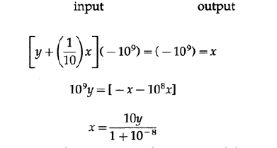
These three examples show what was implicitly mentioned earlier - if there is a feedback loop for the variables used in the task, then it is not necessary to know their values ​​exactly. G. Black’s remarkable idea is based on this: how to build a feedback loop in amplifiers (Figure 20.VIII): as long as the gain is very high, only the resistance of one resistor must be precisely selected, all other parts can be implemented with low accuracy. For the scheme presented in Figure 20.VIII we get the following expressions:



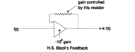
Figure 20.VIII

As can be seen, almost all the measurement uncertainty is concentrated in one resistor of 1/10 nominal, while the transfer coefficient may be inaccurate. Thus, Black's feedback loop allows us to build accurate things from inaccurate parts.



Now you see why I cannot give you an elegant formula suitable for all occasions. It should depend on what calculations are made on specific quantities. Will inaccurate values ​​pass through a feedback loop that compensates for the error, or will errors go out of the system without feedback protection? If the variables do not provide feedback, then it is vital to get their exact values.
So, the awareness of this fact can affect the design of the system! A well-designed system protects you from the need to use a large number of high-precision components. But such design principles are still misunderstood at the moment and require careful study. And the point is not that good designers do not understand this at the level of intuition, it is simply not so easy to apply these principles in the design methods you studied. Good minds still need all the CAD tools that we have developed. The best minds will be able to embed these principles into the studied design methods to make them available out of the box for everyone else.

Let us now turn to another example and principle, which allowed me to get a solution to one important task. I was given a differential equation



It is immediately noticeable that the value of the condition at infinity is indeed the right-hand side of a zero-differential equation, Figure 20.IX

But let's consider the issue of stability. If the value of y at some sufficiently distant point x becomes large enough, then the value of sinh ( y ) becomes much larger, the second derivative takes a large positive value, and the curve fires toward plus infinity. Similarly, if the value of ytoo small, then the curve shoots toward minus infinity. And it doesn't matter at all whether we are moving from left to right or from right to left. Earlier, when I came across a divergent field of directions, I used an obvious trick: I integrated it in the opposite direction and got the exact solution. But in this case, we seem to be on the crest of a sand dune, and as soon as both legs are on the same slope, we fall down.



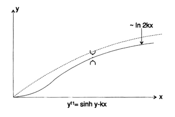
Figure 20.IX

I tried to use the power series decomposition, the power series decomposition that approximates the original curve, but the problem did not go away, especially for large values ​​of k. Neither I nor my friends could offer any adequate solution. Then I went to the task designers and first of all began to challenge the boundary condition at infinity, however, it turned out that this condition is related to the distance measured in the layers of molecules, and at that time, any practically realizable transistor had an almost infinite number of layers. Then I began to challenge the equation, and they again won the argument, and I had to step back into my office and continue to think.

It was an important task related to the design and understanding of the transistors that were being developed at that time. I have always argued that if the task is important and correctly set, then I can find some solution. Therefore, I had no choice, it was a matter of honor.

It took me a few days of thinking to understand that instability was the key to a suitable method. I built a solution of a differential equation on a small interval using a differential analyzer that I had at that time, and if the solution was firing up, it meant that I chose a very large value of the slope, but if it fired down, then I chose too small value. Thus, in small steps, I walked along the ridge of the dune, and as soon as the solution failed on one side, I knew what to do to get back to the ridge. As you see, professional pride is a good assistant when you need to find a solution to an important task in difficult conditions. How easily it was possible to abandon the solution of this problem, to refer to the fact that it is unsolvable, it is incorrectly set or to find any other excuses, but I still believe that important and correctly set tasks provide new useful information. A number of problems related to space charge, which I solved with the help of computational methods, had a similar complexity associated with instability in both directions.

Before telling you the following story, I want to remind you of the Rorschach test, which was popular during my youth. A drop of ink is applied to a sheet of paper, after which it folds in half, and when it is unfolded again, a symmetrical blob is obtained of a rather random shape. The sequence of these blots is shown to the subjects, who are asked to tell what they see. Their answers are used to analyze the "features" of their personality. Obviously, the answers are a figment of their imagination, since essentially the spot has a random form. It's like looking at the clouds in the sky and discuss what they look like. You are discussing only the fruits of your imagination, and not reality, and this in some way reveals something new about yourself and not about clouds. I suppose the inkblot method is no longer used.

And now for the story itself. One day, my psychologist friend from Laboratories Bell built a car that had 12 switches and two light bulbs - red and green. You installed the switches, pressed a button, and then a red or green light came on. After the first subject made 20 attempts, he proposed a theory on how to light a green light bulb. This theory was transmitted to the next victim, after which she also had 20 attempts to propose her theory on how to light a green light bulb. And so on to infinity. The purpose of the experiment was to study how the theories develop.

But my friend, acting in his own style, connected the bulbs to a random source of signals! Once he complained to me that not a single participant in the experiment (and all of them were highly qualified researchers at Bell Laboratories) did not say that there was no pattern. I immediately assumed that none of them was a specialist in statistics or information theory - these two types of specialists are familiar with random events. The check revealed that I was right!

This is a sad consequence of your education. You have lovingly studied how one theory is being replaced by another, but you have not studied how to abandon a beautiful theory and accept chance. That was exactly what was needed: to be ready to admit that the theory just read does not fit, and there is no regularity in the data, pure chance!

I have to stop at this in more detail. The statisticians constantly ask themselves: “What do I mean, does it actually take place, or is it just an occasional noise?”. They developed special testing methods to answer this question. Their answers are not an unambiguous "yes" or "no", but "yes" or "no" with a certain level of confidence. The 90% confidence threshold means that usually out of 10 attempts you will be mistaken only once, provided that all other hypotheses are correct.In this case, one of two things: either you found something that is not (Error of the first kind) or you missed what you were looking for (Error of the second kind). Much more data is needed in order to get a 95% confidence level, and now data collection can be very expensive. Additional data collection also requires additional time and decision making is postponed - this is a favorite trick of people who do not want to take responsibility for their decisions. “More information is needed,” they will tell you.

I absolutely seriously assert that the majority of the modeling produced is nothing more than a Rorschach test. I will quote Jay Forrester’s outstanding practice of control theory: “From the behavior of the system, doubts will arise that will require a revision of the initial assumptions. From the process of processing the initial assumptions about the parts and the observed behavior of the whole, we improve our understanding of the structure and dynamics of the system. This book is the result of several cycles of repeated study, passed by the author. "

How can a non-specialist distinguish this from the Rorschach test? Did he see something simply because he wanted to see it or discovered a new facet of reality? Unfortunately, very often the simulation contains some adjustments that allow you to "see only what you want." This is the path of least resistance, which is why classical science involves a large number of precautions, which in our time are often simply ignored.

Do you think that you are careful enough not to wishful thinking? Let's look at the famous double-blind study, which is a common practice in medicine. At first, doctors found that patients noted an improvement in their condition when they thought they were getting a new medicine, while patients in the control group who know that they are not getting a new medicine do not feel an improvement in their condition. After that, the doctors randomized the groups and gave some patients a placebo so that they could not mislead the doctors. But to his horror, the doctors found that doctors who knew who was taking the medicine and who was not, also found improvements in those who had it and did not find it better for those who hadn’t expected it. As a last resort, doctors began to take a double-blind study method everywhere — until all the data were collected, neither the doctors nor the patients know who is taking the new medicine and who is not. At the end of the experiment, statistics open a sealed envelope and analyze. Doctors who sought honesty, discovered that they themselves are not. Do you do the modeling so much better that you can be trusted? Are you sure that you just did not find what you were trying to find? Self-deception is very common. Do you do the modeling so much better that you can be trusted? Are you sure that you just did not find what you were trying to find? Self-deception is very common. Do you do the modeling so much better that you can be trusted? Are you sure that you just did not find what you were trying to find? Self-deception is very common.

I started chapter 19 by asking the question, why should everyone believe the modeling they did? Now this problem has become more obvious to you. It’s not so easy to answer this question until you have taken a lot more precautions than usual. Remember also that in your high-tech future, you will most likely represent the customer side of the simulation, and you will have to make decisions based on its results. There are no other ways, except modeling, to get an answer to the question “What if ...?”. In Chapter 18, I considered the decisions to be made, rather than being postponed all the time, if the organization is not going to rummage and drift endlessly - I assume that you will be among those who must make a decision.

Simulation is necessary to answer the question “What if ...?”, But it is full of pitfalls, and one should not trust its results simply because large human and hardware resources were involved in order to get beautiful color printouts or curves on an oscilloscope. If you are the one who makes the final decision, then all responsibility lies with you. Collective decisions that lead to a dilution of responsibility are rarely good practice - as a rule, they are a mediocre compromise that lacks the merits of any of the possible ways. Experience has taught me that a decisive boss is a lot better than a blabbing boss. In this case, you know exactly where you are and can continue the work that needs to be done.

The question “What if ...?” Will often arise before you in the future, so you need to properly understand the basics and possibilities of modeling in order to be ready to challenge the results and understand the details where necessary.

To be continued ...

Who wants to help with the translation, layout and publication of the book - write in a personal or mail magisterludi2016@yandex.ru

By the way, we also started the translation of another cool book - "The Dream Machine: The History of Computer Revolution" )