April 6, 2013 at 21:56
Blind Deconvolution - automatic recovery of blurry images
Blurred images are one of the most annoying defects in photography, along with defocused images. Earlier, I wrote about deconvolution algorithms for restoring blurry and defocused images. These relatively simple approaches allow you to restore the original image if the exact trajectory of the smear (or the shape of the blur spot) is known.
In most cases, the lubrication path is assumed to be a straight line, the parameters of which must be set by the user himself - this requires quite painstaking work to select the core, in addition, in real photographs, the lubrication path is far from the line and is an intricate curve of variable density / brightness, the shape of which is extremely difficult to pick by hand.
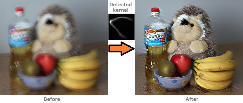
In the last few years, a new direction in the theory of image restoration has been developing intensively - Blind Deconvolution. Quite a lot of work has appeared on this topic, and the active commercial use of the results begins.
Many of you remember the Adobe MAX 2011 conference, at which they just showed the operation of one of the Blind Deconvolution algorithms: Correcting blurry photos in the new version of Photoshop
In this article I want to tell in more detail how this amazing technology works, and also show the practical implementation of SmartDeblur , which now also has this algorithm at its disposal.
Attention, under the cut a lot of pictures!
Part 1. Theory - Restoring Defocused and Blurred Images
Part 2. Practice - Restoring Defocused and Blurred Images
Part 3. Improving Quality - Restoring Defocused and Blurred Images
It is recommended to read at least the first theoretical part, in order to better understand what convolution, deconvolution, Fourier transform, and other terms are. Although I promised that the third part will be the last, but I could not resist and did not tell about the latest trends in the field of image restoration.
I will consider Blind Decovolution as an example of the work of American professor Rob Fergus "Removing Camera Shake from a Single Photograph". The original article can be found on his page: http://cs.nyu.edu/~fergus/pmwiki/pmwiki.php
This is not the newest work, recently there have been many other publications that show better results - but it uses a very complicated mathematics ((for an unprepared reader) in a number of stages, but the basic principle remains the same. Moreover, Fergus’s work is a kind of “classic”, he was one of the first to propose a fundamentally new approach that allowed automatically detecting the lubricant core even for very complex cases.
Take a camera and take a blurry picture - since it doesn’t require much effort :)
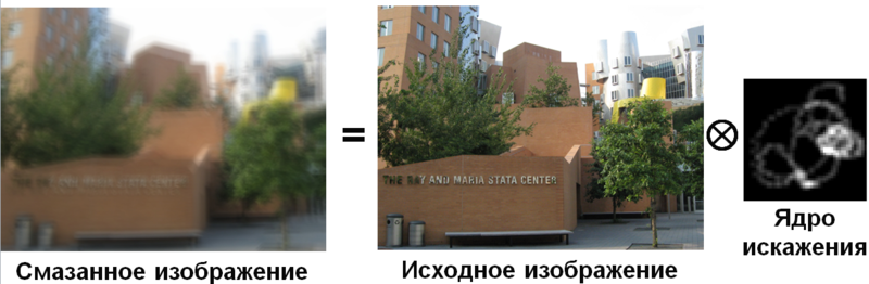
We introduce the following notation:
B is the observed blurred image
K is the blur core (smear path), kernel
L is the original blurry image (hidden)
N is the additive noise
Then the blur process / distortions can be described as the following expression
B = K * L + N
Where the symbol "*" is a convolution operation, not to be confused with ordinary multiplication!
What is convolution can be read in the first part.
In a visual form, this can be represented as follows (omitting the noise component for simplicity):
So what is the most difficult?
Imagine a simple analogy - the number 11 consists of two factors. What are they?
The solutions are endless:
11 = 1 x 11
11 = 2 x 5.5
11 = 3 x 3.667
, etc.
Or, moving on to a visual representation:
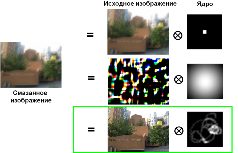
Those. need more information. One of the options for this is to set the objective function - this is a function whose value is the higher (in the simple case), the closer the result is to the desired one.
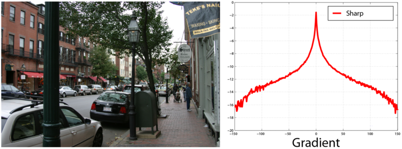
Studies have shown that despite the fact that real images have a large spread in the values of individual pixels, the gradients of these values have the form of a distribution with slowly decreasing boundaries ( Heavy-tailed distribution ). Such a distribution has a peak in the vicinity of zero and, in contrast to the Gaussian distribution, has significantly greater probabilities of large values (such is butter).
This coincides with the intuitive idea that in most cases in real images there are large areas of more or less constant brightness, which end with objects with sharp and medium differences in brightness.
Here is an example of a histogram of gradients for a sharp image:
And for a blurry image:
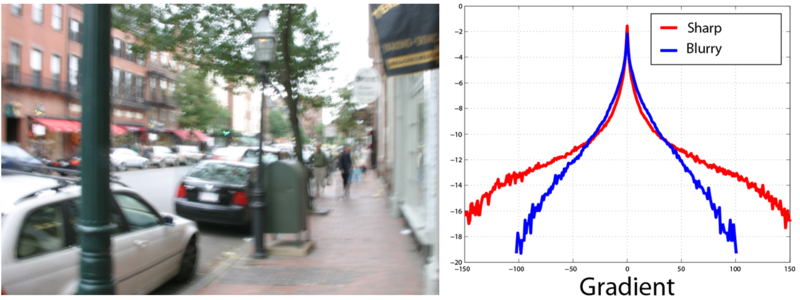
In this way we got a tool that allows us to measure the “quality” of the result in terms of clarity and similarity to a real image.
Now we can formulate the main points for the construction of the completed model:
1. The restrictions imposed by the distortion model B = K * L + N
2. The objective function for the reconstruction result is how similar the histogram of gradients is to the theoretical distribution with slowly decreasing boundaries. We denote it by p (L P )
3. The objective function for the distortion core is positive values and a low proportion of white pixels (since the smear path is usually represented by a thin line). Denote it by p (K).
Combine all this into a common objective function as follows:

Where q (L P ) , q (K) are the distributions obtained by the Variational Bayesian approach
Further, this objective function is minimized by the method of coordinate descent with some additions, which I will not describe because of their complexity and the abundance of formulas - all this can be read in Fergus.
This approach allows improving the quality of the existing core, but they cannot build this core from scratch, because most likely in the process of finding a solution we will fall into one of the local minimums.
First, from the input blurry image, we build a pyramid of images with different resolutions. From the smallest size to the original size.
Next, we initialize the algorithm using a 3 * 3 kernel with one of the simple patterns - a vertical line, a horizontal line, or a Gaussian spot. As a universal option, you can choose the latter - a Gaussian spot.
Using the optimization algorithm described above, we improve the kernel estimate using the smallest image size in the constructed pyramid.
After that, we resize the resulting refined kernel to, say, 5 * 5 pixels and repeat the process with an image of the next size.
Thus, at each step, we slightly improve the core and as a result we get a very accurate trajectory of the lubricant.
Let's demonstrate the iterative construction of the kernel using an example.
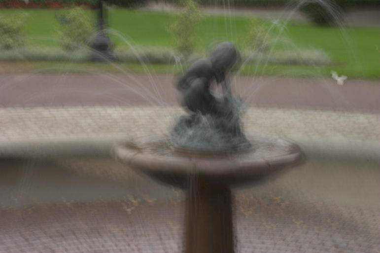
Original Image:
Kernel Refinement Process:
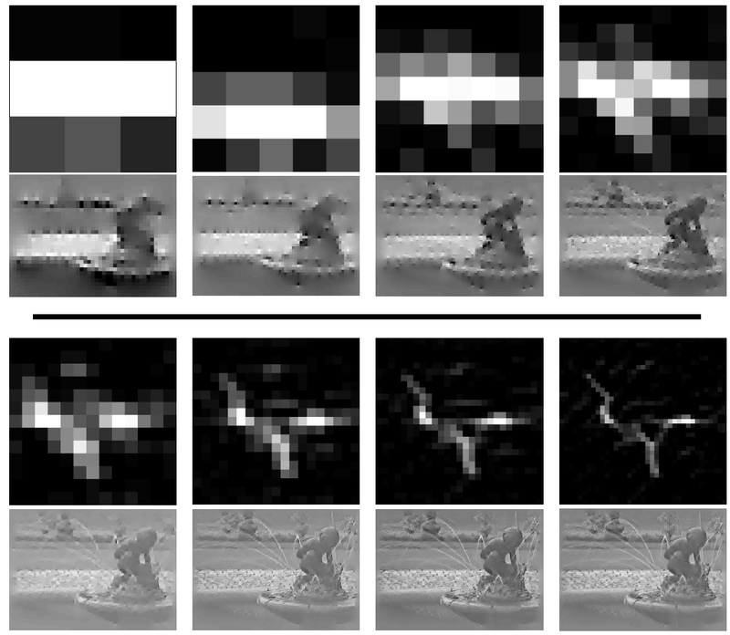
The first and third lines show the kernel rating at each level of the image pyramid.
The second and fourth lines are the estimates of the undistorted image.
Result:
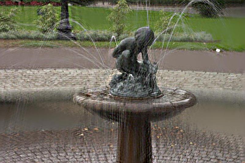
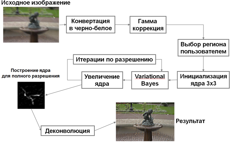
More modern approaches have approximately the same idea of sequential refinement of the kernel, but use more sophisticated versions of the objective function for the reconstruction result and the distortion kernel. In addition, intermediate and final filtering of the resulting core is carried out in order to remove excess noise and fix some errors in the refinement algorithm.
We implemented a similar option and added as a new function in SmartDeblur 2.0 - everything is still free :)
Project address: smartdeblur.net
(Sources and binaries from the previous version can be found on GitHub: github.com/Y-Vladimir/SmartDeblur )
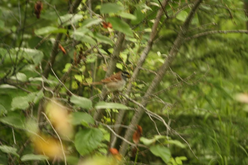
Example of work :
Another example:
And finally, the result of work on the image from the Adobe MAX 2011 conference:
As you can see, the result is almost perfect - almost like Adobe's in their demonstration.
We will increase it later, after we optimize deconvolution and pyramidal construction.
The interface is as follows:
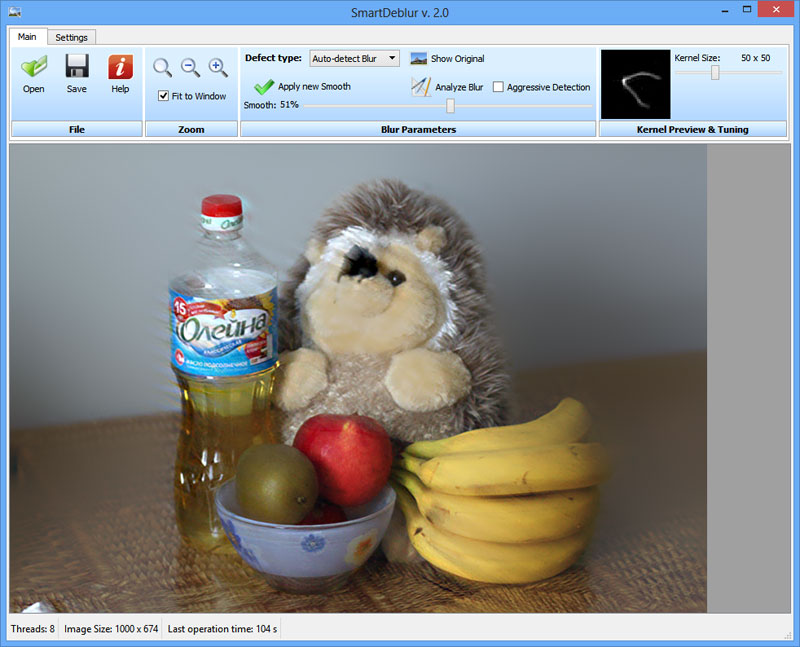
To work with the program, you only need to download the image and click “Analyze Blur” and accept the choice of the whole image - the analysis can take several minutes. If the result does not suit you, you can select another region (select it with the mouse in the image moving it right and down, it is a little not obvious, but so far :)). The right button selects the selection.
The “Agressive Detection” checkbox changes the settings to select only the most important elements of the kernel.
So far, good results are far from being achieved on all images - therefore we will be very happy about the feedback, this will help us improve the algorithms!
Vladimir Yuzhikov (Vladimir Yuzhikov)
In most cases, the lubrication path is assumed to be a straight line, the parameters of which must be set by the user himself - this requires quite painstaking work to select the core, in addition, in real photographs, the lubrication path is far from the line and is an intricate curve of variable density / brightness, the shape of which is extremely difficult to pick by hand.
In the last few years, a new direction in the theory of image restoration has been developing intensively - Blind Deconvolution. Quite a lot of work has appeared on this topic, and the active commercial use of the results begins.
Many of you remember the Adobe MAX 2011 conference, at which they just showed the operation of one of the Blind Deconvolution algorithms: Correcting blurry photos in the new version of Photoshop
In this article I want to tell in more detail how this amazing technology works, and also show the practical implementation of SmartDeblur , which now also has this algorithm at its disposal.
Attention, under the cut a lot of pictures!
Start
This post is a continuation of my post series “Restoring Defocused and Blurred Images”:Part 1. Theory - Restoring Defocused and Blurred Images
Part 2. Practice - Restoring Defocused and Blurred Images
Part 3. Improving Quality - Restoring Defocused and Blurred Images
It is recommended to read at least the first theoretical part, in order to better understand what convolution, deconvolution, Fourier transform, and other terms are. Although I promised that the third part will be the last, but I could not resist and did not tell about the latest trends in the field of image restoration.
I will consider Blind Decovolution as an example of the work of American professor Rob Fergus "Removing Camera Shake from a Single Photograph". The original article can be found on his page: http://cs.nyu.edu/~fergus/pmwiki/pmwiki.php
This is not the newest work, recently there have been many other publications that show better results - but it uses a very complicated mathematics ((for an unprepared reader) in a number of stages, but the basic principle remains the same. Moreover, Fergus’s work is a kind of “classic”, he was one of the first to propose a fundamentally new approach that allowed automatically detecting the lubricant core even for very complex cases.
Distortion model
And so, let's get started.Take a camera and take a blurry picture - since it doesn’t require much effort :)
We introduce the following notation:
B is the observed blurred image
K is the blur core (smear path), kernel
L is the original blurry image (hidden)
N is the additive noise
Then the blur process / distortions can be described as the following expression
B = K * L + N
Where the symbol "*" is a convolution operation, not to be confused with ordinary multiplication!
What is convolution can be read in the first part.
In a visual form, this can be represented as follows (omitting the noise component for simplicity):
So what is the most difficult?
Imagine a simple analogy - the number 11 consists of two factors. What are they?
The solutions are endless:
11 = 1 x 11
11 = 2 x 5.5
11 = 3 x 3.667
, etc.
Or, moving on to a visual representation:
Target function
To get a specific solution, you need to introduce restrictions, somehow describe the model of what we are striving for.Those. need more information. One of the options for this is to set the objective function - this is a function whose value is the higher (in the simple case), the closer the result is to the desired one.
Studies have shown that despite the fact that real images have a large spread in the values of individual pixels, the gradients of these values have the form of a distribution with slowly decreasing boundaries ( Heavy-tailed distribution ). Such a distribution has a peak in the vicinity of zero and, in contrast to the Gaussian distribution, has significantly greater probabilities of large values (such is butter).
This coincides with the intuitive idea that in most cases in real images there are large areas of more or less constant brightness, which end with objects with sharp and medium differences in brightness.
Here is an example of a histogram of gradients for a sharp image:
And for a blurry image:
In this way we got a tool that allows us to measure the “quality” of the result in terms of clarity and similarity to a real image.
Now we can formulate the main points for the construction of the completed model:
1. The restrictions imposed by the distortion model B = K * L + N
2. The objective function for the reconstruction result is how similar the histogram of gradients is to the theoretical distribution with slowly decreasing boundaries. We denote it by p (L P )
3. The objective function for the distortion core is positive values and a low proportion of white pixels (since the smear path is usually represented by a thin line). Denote it by p (K).
Combine all this into a common objective function as follows:
Where q (L P ) , q (K) are the distributions obtained by the Variational Bayesian approach
Further, this objective function is minimized by the method of coordinate descent with some additions, which I will not describe because of their complexity and the abundance of formulas - all this can be read in Fergus.
This approach allows improving the quality of the existing core, but they cannot build this core from scratch, because most likely in the process of finding a solution we will fall into one of the local minimums.
Pyramidal approach
The solution to this problem is an iterative approach to building a distortion core.First, from the input blurry image, we build a pyramid of images with different resolutions. From the smallest size to the original size.
Next, we initialize the algorithm using a 3 * 3 kernel with one of the simple patterns - a vertical line, a horizontal line, or a Gaussian spot. As a universal option, you can choose the latter - a Gaussian spot.
Using the optimization algorithm described above, we improve the kernel estimate using the smallest image size in the constructed pyramid.
After that, we resize the resulting refined kernel to, say, 5 * 5 pixels and repeat the process with an image of the next size.
Thus, at each step, we slightly improve the core and as a result we get a very accurate trajectory of the lubricant.
Let's demonstrate the iterative construction of the kernel using an example.
Original Image:
Kernel Refinement Process:
The first and third lines show the kernel rating at each level of the image pyramid.
The second and fourth lines are the estimates of the undistorted image.
Result:
Flowchart
It remains to put everything together and describe the whole algorithm:More modern approaches have approximately the same idea of sequential refinement of the kernel, but use more sophisticated versions of the objective function for the reconstruction result and the distortion kernel. In addition, intermediate and final filtering of the resulting core is carried out in order to remove excess noise and fix some errors in the refinement algorithm.
Practical implementation
Probably the most interesting thing is to play around with the Blind Deconvolution algorithm live on real images!We implemented a similar option and added as a new function in SmartDeblur 2.0 - everything is still free :)
Project address: smartdeblur.net
(Sources and binaries from the previous version can be found on GitHub: github.com/Y-Vladimir/SmartDeblur )
Example of work :
Another example:
 |  |
 |
And finally, the result of work on the image from the Adobe MAX 2011 conference:
 |  |
 |
As you can see, the result is almost perfect - almost like Adobe's in their demonstration.
Technical details
So far, the maximum size of the processed image is set to 1200 * 1200. This is due to the fact that algorithms consume a lot of memory. Even in an image of 1000 pixels - more than a gigabyte. Therefore, a size restriction has been introduced.We will increase it later, after we optimize deconvolution and pyramidal construction.
The interface is as follows:
To work with the program, you only need to download the image and click “Analyze Blur” and accept the choice of the whole image - the analysis can take several minutes. If the result does not suit you, you can select another region (select it with the mouse in the image moving it right and down, it is a little not obvious, but so far :)). The right button selects the selection.
The “Agressive Detection” checkbox changes the settings to select only the most important elements of the kernel.
So far, good results are far from being achieved on all images - therefore we will be very happy about the feedback, this will help us improve the algorithms!
--Vladimir Yuzhikov (Vladimir Yuzhikov)