Solving the problem of finding the camera’s installation angles over the road using different methods in Wolfram Mathematica. Part 1
Formulation of the problem
There is a system located above the roadway, which includes a video camera. Known camera resolution and viewing angles. Concerning the roadway, the video camera is installed as follows: from above above any of the lanes, to the side of the roadway no more than 3 meters from the edge of the nearest controlled lane. The number of simultaneously controlled lanes is not more than 4. The video camera takes photographs of the control zone with a certain frame rate. All frames made are input to the license plate recognition system. The result of driving a vehicle (hereinafter referred to as “TS”) is a track with the coordinates of the center of the vehicle license plate frame in the form:
x11 y11 x12 y12 … x1i y1i … x1n y1nThe result of driving several vehicles is a track file in the form:
x11 y11 x12 y12 … x1i y1i … x1n y1nx21 y21 x22 y22 … x2i y2i … x2n y2n...xi1 yi1 xi2 yi2 … xii yii … xin yin...xn1 yn1 xn2 yn2 … xni yni … xnn ynnExample of a track file:
1420 23 1399 44 1377 62 1351 82417 327 368 359 313 392 119 500 48 5402300 62 2291 91 2275 125 2267 159 2254 1972298 114 2263 223 2199 413 2180 470 2158 532It is necessary, having a file with the structure described above, to determine the angle of the camera relative to the trajectories of vehicles and the rotation of the camera relative to the edge of the curb.
Data import
We import the data we will work with.
Our file lies in the directory from which the laptop is launched (Mathematica document), called the file recdat.txt. To import, we introduce:
file = Import[NotebookDirectory[] <> "recdat.txt", "Table"];file- the variable into which the file NotebookDirectory[]is imported - returns the directory where the laptop is located in the form of a string <>- an abbreviated record of the function connecting the lines "recdat.txt"- a string indicating the name of the file with tracks "Table"- the option of the Import [] function, indicating that this file must be imported in the form of a table, respectively, the file variable will have the type of the table (list) The symbol
;at the end of the line indicates that Mathematica will not output the result of the described function after its execution.Pressing Shift + Enter will import our file.
In order to see exactly how the data was imported, you need to enter file and press Shift + Enter, but for a more visual display of information, we use the following function:
TableForm[file]1420 23 1399 44 1377 62 1351 82 417 327 368 359 313 392 119 500 48 5402300 62 2291 91 2275 125 2267 159 2254 1972298 114 2263 223 2199 413 2180 470 2158 532TableForm[list]- performs output with list elements located in an array of rectangular elements. We determine the constants that specify the resolution of the camera and angles overview:
Xlen = 2360; (*Горизонтальное разрешение камеры*)Ylen = 1776; (* Вертикальное разрешение камеры*)Xang = 14; (*Горизонтальный угол обзора камеры*)Yang = Xang*3/4; (*Вертикальный угол обзора камеры*)Determine the number of tracks in the file:
length = Length[file];Length[list]- returns the number of elements in the one-dimensional list list or the number of dimensions in the case of a multi-dimensional listExpanding imported data into a structure
Imported data is a structure that is not convenient to work with in Mathematica. It will be much more convenient to work with them if you expand them into a structure in the form of a three-dimensional list, where an element with index i, j consists of two elements - the x- and y-coordinates of the center of the license plate, with i being the serial number of the license plate, and j - serial number of the track point for the i-th license plate.
A small digression from the topic:
In Mathematica, the same action can be done in different ways, because The environment includes a huge set of various functions; the same action can be done using a loop, or it can be done using a special Mathematica function. As a rule, the execution time of an action aimed at the same functionality is shorter when it is performed using the standard Wolfram function than when it is performed using a self-written loop. The execution time of a function or set of functions helps determine the function Timing[].To create a list into which we will decompose the structure, we first declare the variable as a list:
num = {};To expand our data into the structure, we write a loop:
Do[num = Append[num, Partition[file[[i]], 2]], {i, length}]Do[action, {condition for executing the loop}] Append[list,element]- adds an element to the end of the list Partition[list,n]- splits the list into non-overlapping parts with a length n If the number of elements in the list is not completely divided by n, then the last k (kfile[[i]]- returns the i element of the list Now, let's turn to the function we already know, and see what the structure looks like, convenient for further processing:
TableForm[num, TableSpacing -> {3, 4}]
TableSpacing -> {3, 4}- sets the indentation between the elements of the list when displayingGetting track equations
In the particular case, track points must be linearized. “In private” - because the data considered above was obtained on a direct road, where vehicles move at high speeds, and during the passage of the control zone physically at that speed they cannot move along trajectories that are very different from straight lines.
We will write down the equations of motion of the vehicle in the list. To do this, we first declare it:
numeq = {};And we write a function to determine the equations of motion of the vehicle through the control zone. It is necessary to say here that the origin in the frame is the upper left corner of the frame, so:
Do[numeq = Append[numeq, Fit[num[[i]], {1, x}, x]], {i, length}]Fit [data, funs, vars] - for a list of data, data looks for the least squares approximation in the form of a linear combination of funs functions of the vars variables. Data data can be of the form {{x1, y1, ..., f1}, {x2, y2, ..., f2}, ...}, where the number of coordinates x, y, ... is equal to the number of variables in the vars list . Also, data data can be represented in the form {f1, f2, ...} with one coordinate taking values 1,2, ... The funs argument can be any list of functions that depend only on vars objects.
In our case, for each i-th element of the multidimensional list num containing a two-dimensional array of points - the centers of the license plate of the vehicle - we determine by a least square method a function of the form kx + b closest to the existing set of points.
The result of this cycle is a list of approximately the following:
{1167.11 - 0.803101 x, 568.193 - 0.571513 x, 6110.1 - 2.62293 x, 6471.36 - 2.75496 x, 1199.09 - 0.812067 x, 2491.96 - 1.29425 x, 1121.33 - 0.787616 x, 2933.43 - 1.75218 x, 625.959 - 0.609492 x, 2512.3 - 1.30408 x, 7805.9 - 3.3897 x, 881.413 - 0.698268 x, 2651.99 - 1.3463 x, 6140.19 - 2.61239 x, 2594.17 - 1.27645 x, 557.83 - 0.587095 x, 1195.29 - 0.82697 x, 6346.13 - 2.73884 x, 6887.01 - 2.92561 x, 2377.62 - 1.26743 x, 3241.53 - 1.72441 x, 1424.49 - 0.846298 x, 1218.75 - 0.83174 x, 7203.35 - 3.089 x, 5420.94 - 2.28441 x, 2500.74 - 1.29295 x, 2402.61 - 1.25934 x, 6760. - 2.89566 x, 1175.7 - 0.794353 x, 1117.2 - 0.77705 x, 7066.9 - 3.00537 x, 2346.99 - 1.24765 x, 2698.98 - 1.39178 x, 1277.43 - 0.849703 x, 633.372 - 0.61772 x, 2578.56 - 1.3082 x, 2952.21 - 1.47007 x, 1107.8 - 0.7861 x, 2352.46 - 1.24075 x, 2326.56 - 1.23348 x...}Graphical representation of data and lines from a list of equations
After receiving the equations, we can display on the graph all the points we have and the corresponding equations.
Mathematica has a function
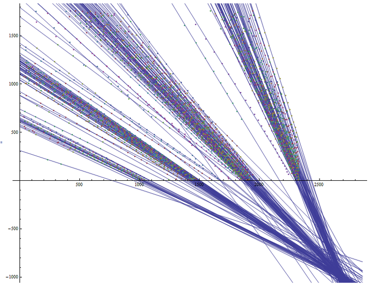
ListPlot[]for displaying a list of points on a graph , and a function for displaying functions Plot[]. In order to display a graph with points and function graphs on one graph, or to override the graph parameters, there is a function Show[]. We will write these functions for our case: eqlineplot = Plot[numeq[[Range[length]]], {x, 0, Xlen}];numplot = ListPlot[num[[Range[length]]]];Show[ eqlineplot, numplot, AspectRatio -> 3/4, Frame -> False, PlotRange -> {{0, Xlen}, {0, Ylen}}]And the result of its execution:

This graph is reversible with respect to the OX axis, as his point of origin is in the lower left edge, and not like the camera in the upper left. But this does not prevent us from understanding that the lines intersect somewhere in the vicinity of one point - the point from which we will continue to count the angles. Below is a graph with slightly changed drawing areas, which shows the intersection of lines in the vicinity of one point: Let's
take a closer look at the function records:
eqlineplot = Plot [numeq [[Range [length]]], {x, 0, Xlen}];
Plot [list of functions that will be displayed on the chart,
{variable relative to which the functions are constructed,
its minimum value,
its maximum value}]
Range [imax] - generates a list of numerical elements {1, 2, ..., imax}
Show [
eqlineplot,
numplot,
AspectRatio -> 3/4, Frame -> False,
PlotRange -> {{0, Xlen}, {0, Ylen}}]
AspectRatio -> 3/4 - set the aspect ratios of the
PlotRange -> {{0 , Xlen}, {0, Ylen}} set the range of graphs to be drawn on the coordinates X and Y
Frame -> False - tell Mathematica that there is no need to draw a frame around the graph.
What's next?
In the sequel, if it seems interesting and necessary to you, I will talk about several methods for finding the intersection points of graphs, introduce you to statistical data processing and data analysis using the example of the problem under consideration.