Overview and Comparison of Gateway Quantum Software Platforms
Hi, Habr! I present to your attention the translation of the article "Overview and Comparison of the Gate Level Quantum Software Platforms" by Ryan LaRose.
Quantum computers are available for use in the cloud infrastructure, but at the same time, the recent rapid growth of quantum software platforms can be overwhelming for those who will decide what to use. This article offers a current picture of the rapidly growing landscape of quantum computing by comparing four software platforms — Forest (pyQuil), QISKit, ProjectQ and the Quantum Development Kit — which allow researchers to use real and simulated quantum devices. This analysis covers the requirements and installation, the syntax of the language on the example of programs, support at the library level and the capabilities of the quantum simulator for each platform. For platforms with quantum computer support, we compare hardware, quantum assembler languages, and quantum compilers.
Content
I. Introduction
II. Software platforms
A. pyQuil
B. QISKit
C. ProjectQ
D. Quatum Development Kit
III. Comparison
A. Library Support
B. Quantum Hardware
C. Quantum Compilers
D. Simulator Performance
E. Features
IV. Discussion and conclusions
References
Appendix A. Other software platforms
Appendix B. Testing the performance of the simulator
Appendix C. Sample program: Teleportation scheme
I. Introduction
Quantum programming languages were considered at least two decades ago [1-3], but they were mostly theoretical and without existing equipment. Quantum computers are now a reality, and there are quantum programming languages that allow anyone who has access to the Internet to use them. A sufficient number of researchers, both in industry and in academic circles, have created small quantum devices that operate on a circuit model of quantum computing. These computers are small, noisy and not as powerful as modern classic computers. But they are emerging, growing steadily and foreshadowing future unimaginably large computational powers for the tasks of chemistry [4, 5], machine learning [6, 7], optimization [8], financial sphere [9] and more [10]. These devices are a test bench for training the next generation of quantum software engineers to solve the currently existing classically complex problems of computer technology. Indeed, cloud quantum computing has already been used to calculate the deuteron coupling energy [11] and test subroutines in machine learning algorithms [12, 13].
Recently, there has been a rapid growth of software for quantum computing in a wide variety of classical computer languages. A list of open source projects with more than fifty is available in [14], and a list of quantum computer simulators is available in [15]. This huge number of programs that positively reflect the growth in the field makes it difficult for students and researchers to decide which software package to use in order not to get lost in the documentation or be shocked by the necessary basic knowledge.
This article is expected to provide a brief overview and comparison of the main software platforms for general-purpose quantum computing at the gate level. Four were selected from the long list: three that provide the user with the ability to connect to real quantum devices - pyQuil from Rigetti [16], QISKit from IBM [17] and ProjectQ from ETH Zurich [18, 19], and one with similar functionality, but without the current ability to connect to a quantum computer - Microsoft's Quantum Development Kit [20]. In favor of the choice of these platforms was the ability to connect to a real quantum device. Because of this, and for the sake of brevity, a number of respectable programs are intentionally omitted. Some of them are mentioned in Annex A .
At the moment, the main goal is to present a picture of the landscape of quantum computation arising from these four platforms. In Section II, we will look at each platform in turn, discussing requirements and installation, documentation and tutorials, language syntax and quantum equipment. Section III offers a detailed comparison of the platforms. It includes: the support level libraries quantum algorithms III A , hardware support in quantum III B , compilers quantum schemes III C and quantum computer simulations III D . Section IV discusses some subjective comments about each platform. Appendix Acontains information about other quantum software, Appendix B contains detailed information about testing a quantum circuit simulator, and Appendix C shows the code for a quantum teleportation scheme in each of the four languages for side-by-side comparison.
Ii. Software platforms
Figure 1 shows various quantum computers and software used to connect to devices. Currently, four software platforms allow you to connect to four different quantum computers - one from Rigetti, an 8-qubit quantum computer, you can connect using pyQuil [41]; and three from IBM, with the largest available number of 16 qubits, which can be connected using QISKit or ProjectQ. In addition, IBM offers a fourth 20-qubit quantum computer, but this device is only available to members of the IBM Q Network [42]: a group of companies, universities, and national laboratories interested in and investing in quantum computing. Figure 1 also shows the quantum computers of companies like Google, IBM and Intel that were announced.
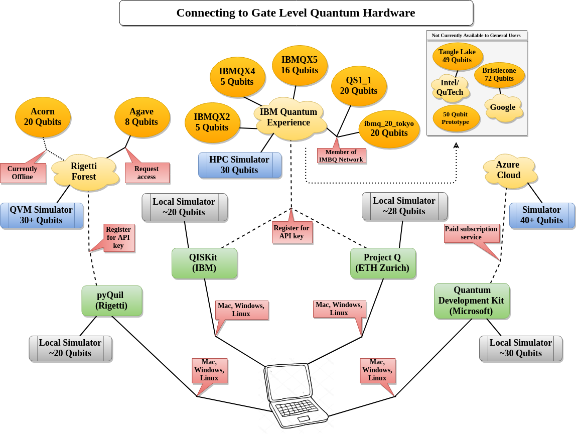
Figure 1. A schematic diagram showing how to connect a personal computer to a quantum computer used at the gate level. Starting from a personal computer (bottom center), the green nodes show software that can be installed on a user's personal computer. Gray nodes indicate that simulators are running locally (that is, on the user's computer). Dotted lines indicate API / cloud connections to company resources shown in yellow "clouds". Quantum simulators and used quantum computers provided by these cloud resources are shown in blue and gold, respectively. Red boxes indicate requirements on the selected method. For example, to connect to Rigetti Forest and use the Agave 8 qubit quantum computer, you must download and install pyQuil (available on MacOS, Windows and Linux), register on the Rigetti website to get the API key, and then request access to the device via the online form. Notes: (i) The quantum virtual machine Rigetti requires elevation for more than 30 qubits, (ii) local simulators depend on the user's computer, therefore the numbers are approximate, and (iii) quantum computers that have been announced, but which currently unavailable for regular users.
The technology of quantum equipment is changing rapidly. It is very likely that new computers will appear by the end of the year, and in two or three years this list may be completely outdated. However, what remains is the software used to connect to this technology. It would be very simple to use new quantum computers, changing just a few lines of code, without actually changing the syntax used to generate or run a quantum scheme. For example, in QISKit, you just need to change the name of the backend device when executing the schema:
execute(quantum_circuit, backend="name", ...)Listing 1. The string "name" points to the backend device for running quantum programs using QISKit. When the future quantum computers are released, the implementation on the new hardware will be as simple as changing the name.
Although the software also changes with the release of the new version [43], these are, for the most part, relatively minor syntax changes that do not significantly change the functionality of the software.
In this section, we will examine each of the four platforms in turn, discussing requirements and installation, documentation and manuals, language syntax, quantum language, quantum equipment, and simulator capabilities. This review is not intended to complete language learning, but it gives the reader an understanding of each platform before diving into one (or more) of the selected platforms. Current analysis includes sufficient information to run algorithms on quantum computers. However, the reader, when he chooses a specific platform, is sent to the special documentation for full information. Links to documentation and tutorial sources for each software package have been added. It is also assumed that there is a basic knowledge of quantum computing, for which there are now many good references [21, 22].
All code snippets and programs included in this document were tested and run on a Dell XPS 13 Developer Edition laptop running Linux Ubuntu 16.04 LTS, the full specifications of which are listed in [23]. Although all software packages work in all three major operating systems, according to the author’s experience, it is much easier to install and use software on the platform on which it was developed. On Linux Ubuntu, there were no difficulties or unusual error messages when installing these software packages.
| pyQuil | QISKit | ProjectQ | QDK | |
|---|---|---|---|---|
| Institution | Rigetti | Ibm | ETH Zurich | Microsoft |
| First release | v0.0.2 on Jan 15, 2017 | 0.1 on March 7, 2017 | v0.1.0 on Jan 3, 2017 | 0.1.1712.901 on Jan 4, 2018 (pre-release) |
| Current Version | v1.9.0 on June 6, 2018 | 0.5.4 on June 11, 2018 | v0.3.6 on Feb 6, 2018 | 0.2.1802.2202 on Feb 26, 2018 (pre-release) |
| Open Source? | ✅ | ✅ | ✅ | ✅ |
| License | Apache-2.0 | Apache-2.0 | Apache-2.0 | MIT |
| Homepage | Home | Home | Home | Home |
| Github | Git | Git | Git | Git |
| Documentation | Docs , Tutorials ( Grove ) | Docs , Tutorial Notebooks , Hardware | Docs , Example Programs , Paper | Docs |
| OS | Mac, Windows, Linux | Mac, Windows, Linux | Mac, Windows, Linux | Mac, Windows, Linux |
| Requirements | Python 3, Anaconda (recommended) | Python 3.5+, Jupyter Notebooks (for tutorials), Anaconda 3 (recommended) | Python 2 or 3 | Visual Studio Code (strongly recommended) |
| Classical Language | Python | Python | Python | Q # |
| Quantum Language | Quil | Openqasm | none / hybrid | Q # |
| Quantum Hardware | 8 qubits | IBMQX2 (5 qubits), IBMQX4 (5 qubits), IBMQX5 (16 qubits), QS1_1 (20 qubits) | no dedicated hardware, can connect to ibm backends | none |
| Simulator | ∼20 qubits locally, 26 qubits with most API keys to QVM, 30+ w / private access | ∼25 qubits locally, 30 through cloud | ∼28 qubits locally | 30 qubits locally, 40 through Azure cloud |
| Features | Generate Quil code, Slack channel, algorithms in Grove, topology-specific compiler, noise capabilities in simulator, community | Generate QASM code, topology specific compiler, community channel, circuit drawer, ACQUA library | Draw circuits, connect to IBM backends, multiple library plug-ins | Built-in algorithms, example algorithms |
A. pyQuil
pyQuil — это библиотека для языка Python с открытым исходным кодом, разработанная Rigetti для создания, анализа и выполнения квантовых программ. Она построена на основе языка Quil — открытый язык квантовых инструкций (или просто квантовый язык), специально разработанного для ближайших перспективных квантовых компьютеров и основанного на общей модели классической/квантовой памяти [24] (это означает, что для памяти доступны как кубиты, так и классические биты). pyQuil — это одна из основных библиотек, разрабатываемых в Forest, которая является ключевой платформой для всего программного обеспечения Rigetti. Forest также включает Grove и Reference QVM, которые будут описаны далее.
a. Требования и установка
Чтобы установить и использовать pyQuil, требуется Python 2 или 3 версии, хотя настоятельно рекомендуется Python 3, поскольку будущие разрабатываемые функции будут поддерживать только Python 3. Кроме того, дистрибутив Python Anaconda рекомендуется для различных зависимостей модуля Python, хотя это не обязательно.
Самый простой способ установки pyQuil — использовать команду диспетчера пакетов Python. В командной строке Linux Ubuntu вводится
pip install pyquilдля успешной установки программного обеспечения. В качестве альтернативы, если Anaconda установлен, pyQuil можно установить, набрав
conda install −c rigetti pyquilв командной строке. Другой альтернативой является загрузка исходного кода из репозитория git и установкой программного обеспечения. Для этого нужно ввести следующие команды:
git clone https://github.com/rigetticomputing/pyquil
cd pyquil
pip install −e
Этот последний метод рекомендуется для всех пользователей, которые могут внести свой вклад в pyQuil. Более подробную информацию смотрите в руководстве по вкладам GitHub.
b. Документация и учебные пособия
pyQuil имеет отличную документацию, размещенную в Интернете, с введением в область квантовых вычислений, инструкциями по установке, базовыми программами и гейтовыми операциями, симулятором, известным как квантовая виртуальная машина (QVM), реальный квантовый компьютер и язык Quil с компилятором. Загрузив исходный код pyQuil с GitHub, вы также получите папку с примерами в Jupyter-тетрадях, обычных примеров на Python и программой , которая может запускать текстовые документы, написанные в Quil, используя квантовую виртуальную машину. Наконец, упоминем Grove, набор квантовых алгоритмов, построенных с использованием pyQuil и среды Rigetti Forest.
c. Синтаксис
Синтаксис pyQuil очень простой и практичный. Основным элементом для записи квантовых схем является программа и может быть импортирована из . Гейтовые операции можно найти в . Модуль позволяет запускать квантовые схемы на виртуальной машине. Одна из приятных особенностей pyQuil заключается в том, что регистры кубитов и классические регистры не обязательно должны быть определены априори и могут быть выделены в памяти динамически. Кубиты в регистре кубитов упоминаются индексами (0, 1, 2, ...) и аналогично для бит в классическом регистре. Таким образом, схему случайного генератора можно записать следующим образом:
# random number generator circuit in pyQuilfrom pyquil.quil import Program
import pyquil.gates as gates
from pyquil import api
qprog = Program()
qprog += [gates.H(0), gates.MEASURE(0, 0)]
qvm = api.QVMConnection()
print(qvm.run(qprog))
Листинг 2. Код pyQuil для генератора случайных чисел.
В первых трех строках импортируется минимум, необходимый для объявления квантовой схемы/программы (строка 2), для выполнения гейтовых операций над кубитами (строка 3) [44] и для выполнения схемы (строка 4). В строке 6 создается квантовая программа, а в строках 7-8 передается ей список инструкций: сначала подействуем гейтом Адамара над кубитом под индексом 0, затем измеряем этот же кубит в классический бит под индексом 0. В строке 10 устанавливается соединение с QVM, а в 11 запускается и выводится результат нашей схемы. Эта программа печатает стандартный вывод pyQuil в виде списка списков целых чисел: в нашем случае — или . В общем, количество элементов во внешнем списке — это количество выполненных испытаний. Целочисленные числа во внутренних списках представляют собой окончательные измерения в классическом регистре. Поскольку мы провели только одно испытание (это указано как аргумент в , который по умолчанию установлен в единицу), мы получаем только один внутренний список. Поскольку в классическом регистре мы имели только один бит, то мы получаем только одно целое число.
d. Квантовый язык
Quil — это язык квантовых инструкций или просто квантовый язык, который передает команды квантовому компьютеру. Это аналогично ассемблеру на классических компьютерах. Основа синтаксиса Quil — это , где является квантовым вентилем, который применяется к кубиту, индексированным (0, 1, 2, ...). pyQuil имеет функцию для генерации кода Quil из заданной программы. Например, в вышеупомянутом генераторе квантовых случайных чисел мы могли бы добавить строку:
print(qprog)в конце для получения кода Quil-схемы, который показан ниже:
H0
MEASURE 0 [0]
Листинг 3. Код Quil для генератора случайных чисел.
Возможно, если кто-то станет разбираться в Quil, написать квантовые схемы в текстовом редакторе на языке Quil, а затем выполнить схему на QVM с помощью программы . Можно также модифицировать , чтобы запустить схему на QPU. Заметим, что компилятор pyQuil (также называемый компилятором Quil в документации) преобразует заданную схему в код Quil, который может понять реальный квантовый компьютер. Мы обсудим это подробнее в разделе III C.
f. Квантовое аппаратное оборудование
Rigetti имеет квантовый процессор, который может использоваться теми, кто запросил доступ. Чтобы запросить доступ, вы должны посетить веб-сайт Rigetti и указать полное имя, адрес электронной почты, название организации и описание основания для доступа к QPU. Как только это будет сделано, представитель компании обратится по электронной почте, чтобы запланировать время, чтобы предоставить пользователю доступ к QPU. Преимущество этого процесса планирования в отличие от системы очередей QISKit, которая будет обсуждаться далее, заключается в том, что многие задания могут выполняться в распределенном временном интервале с детерминированными временем выполнения, что является ключевым для вариационных и гибридных алгоритмов. Эти типы алгоритмов отправляют данные в обратном и прямом направлении между классическими и квантовыми компьютерами — необходимость ждать очереди делает этот процесс значительно дольше. Недостатком (возможно) является то, что задания не могут выполняться в любое время, когда доступен QPU и необходимо указать, и согласиться на конкретное время.
По опыту автора сотрудники готовы помочь, и процесс, как правило, успешен. Актуальное устройство, топология которого показана на Фигуре 2, состоит из 8 кубит со связанностью ближайшего соседа. Мы рассмотрим этот компьютер более подробно в разделе III B.
g. Симулятор
Квантовая виртуальная машина (QVM) является основной утилитой, используемой для выполнения квантовых схем. Это программа, написанная для запуска на классическом процессоре, получает код Quil и моделирует развитие процесса на реальном квантовом компьютере. Чтобы подключиться к QVM, необходимо бесплатно зарегистрировать ключ API на https://www.rigetti.com/forest, указав имя и адрес электронной почты. Затем придёт электронное письмо, содержащее ключ API и идентификатор пользователя, который должен быть настроен при запуске:
pyquil−config−setupв командной строке (после установки pyQuil, конечно). Затем появится запрос на ввод ключей из электронной почты.
Согласно документации, большинство ключей API предоставляют доступ к QVM до 30 кубит, и можно запросить доступ к большему количеству кубит. Ключ API автора дает доступ к 26 кубитам (обновления не запрашивались).
Кроме того, библиотека Forest содержит локальный симулятор, написанный на Python и с открытым исходным кодом, называемый как Reference QVM. Он не такой производительный, как QVM, но пользователи могут запускать схемы с количеством кубитов, ограниченными количеством памяти на локальных машинах. Как правило, схемы с количеством кубит меньше 20-ти возможно запустить на широком кругу оборудовании. Reference QVM должен устанавливаться отдельно, что может быть сделано с помощью :
pip install referenceqvmЧтобы использовать Reference QVM вместо QVM, просто импортируйте из вместо pyQuil:
import referenceapi.api as api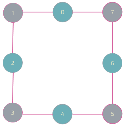
Figure 2. Schematic diagram showing the topology (connectivity) of an 8-qubit Agave QPU Rigetti. Qubits are marked with integers 0, 1, ..., 7, and the lines connecting qubits indicate that a two qubit operation can be performed between these qubits. For example, we can execute Controlled- over qubits 0 and 1, but not between 0 and 2. To do this, the Quil compiler transforms Controlled-(0, 2) in operations that QPU can perform. This diagram is taken from the pyQuil documentation.
B. QISKit
Quantum Information Software Kit, или QISKit, представляет собой комплект разработчика программного обеспечения (SDK) с открытым исходным кодом для работы с квантовым языком OpenQASM и квантовыми процессорами в платформе IBM Q. Он доступен для языков Python, JavaScript и Swift, но здесь мы обсуждаем только версию Python.
a. Требования и установка
QISKit доступен в MacOS, Windows и Linux. Для установки QISKit требуется Python 3.5+. Дополнительные полезные, но не обязательные компоненты — это Jupyter Notebooks для учебных пособий и дистрибутив Python Anaconda 3, в которым присутствуют все необходимые зависимости.
Самый простой способ установить QISKit — это использовать менеджер пакетов pip для Python. В командной строке, для установки программного обеспечение, введем:
pip install qiskitОбратите внимание, что автоматически обрабатывает все зависимости и всегда будет устанавливать последнюю версию. Пользователи, которые могут быть заинтересованы внести вклад в QISKit, могут установить исходный код, введя в командной строке следующее, предполагается, что git установлен:
git clone https://github.com/QISKit/qiskit−core
cd qiskit−core
python −m pip install −e
Для получения информации о вкладах смотрите в онлайн-документации руководства по вкладам на GitHub.
b. Документация и учебные материалы
Документацию QISKit можно найти в Интернете по адресу https://qiskit.org/documentation/. В нем содержатся инструкции по установке и настройке, примеры программ и подключение к реальным квантовым устройствам, организация проекта, обзор QISKit и документация для разработчика. Базовая информация о квантовых вычислениях также может быть найдена для пользователей, которые являются новичками в этой области. Очень хороший ресурс — это ссылка на SDK, где пользователи могут найти информацию о документации по исходному коду.
QISKit также содержит большое количество учебных пособий в отдельном репозитории GitHub (аналогично pyQuil и Grove). К ним относятся запутанные состояния; стандартные алгоритмы, такие как Дойча-Йожа, алгоритм Гровера, оценка фазы и квантовое преобразование Фурье; также более сложные алгоритмы, такие как решение квантовой вариационной задачи на собственные значения и приложение к фермионным гамильтонианам; и даже некоторые забавные игры, такие как квантовый «морской бой». Кроме того, библиотека ACQUA (Algorithms and Circuits for QUantum Applications) содержит многопрофильные алгоритмы для химии и искусственного интеллекта с многочисленными примерами.
Существует также очень подробная документация для каждого из четырех квантовых бэкендов, содержащих информацию о связности, времени когерентности и времени применения гейта. Наконец, упомянем веб-сайт IBM Q experience и руководства пользователя. Веб-сайт содержит графический интерфейс для квантовой схемы, в котором пользователи могут перетаскивать гейты на схему, что полезно для изучения квантовых схем. Руководства пользователя содержат больше инструкций по квантовым вычислениям и языку QISKit.
c. Синтаксис
На синтаксис QISKit можно посмотреть в следующей примерной программе. Здесь, в отличие от pyQuil, нужно явно выделить квантовые и классические регистры. Ниже показана программа для схемы случайных чисел в QISKit:
# random number generator circuit in QISKitfrom qiskit import QuantumRegister, ClassicalRegister, QuantumCircuit, execute
qreg = QuantumRegister(1)
creg = ClassicalRegister(1)
qcircuit = QuantumCircuit(qreg , creg)
qcircuit.h(qreg[0])
qcircuit.measure(qreg[0], creg[0])
result = execute(qcircuit, ’local qasm simulator’).result()
print(result.get_counts())
Листинг 4. Код QISKit для генератора случайных чисел.
В строке 2 импортируются инструменты для создания квантовых и классических регистров, квантовой схемы и функции для выполнения этой схемы. Затем мы создаем квантовый регистр с одним кубитом (строка 4), классический регистр с одним битом (строка 5) и квантовую схему с обоими этими регистрами (строка 6). Теперь, когда схема создана, мы начинаем подавать инструкции: в строке 8 применяем гейт Адамара к нулевому кубиту в нашем квантовом регистре (который является единственным кубитом в квантовом регистре); в строке 9 измеряем этот кубит в классический бит, индексированный нулем в нашем классическом регистре (который является единственным в классическом регистре) [45]. Теперь, когда квантовая схема построена, выполним ее в строке 11 и распечатаем результат в строке 12. Посредством вывода мы получаем «подсчеты» схемы, то есть словарь выходных данных и сколько раз получали каждый результат. Для нашего случая единственными возможными выходами являются 0 или 1, а пример вывода вышеуказанной программы — , что указывает на то, что мы получили 532 экземпляра 0 и 492 экземпляра 1. (По умолчанию количество циклов для запуска схемы, называемое в QISKit, равно 1024.)
d. Квантовый язык
OpenQASM (открытый язык квантового ассемблера [25], который мы можем назвать просто QASM) — это квантовый язык, который предоставляет инструкцию для реальных квантовых устройств, аналогичных ассемблеру на классических компьютерах. Основой синтаксиса QASM является , где задает операцию квантового вентиля, а — кубит. QISKit имеет функцию для генерации кода QASM из схемы. В приведенном выше примере схемы случайных чисел мы могли бы добавить строку.
print(qcircuit.qasm())в конце для получения кода QASM для схемы, показанной ниже:
OPENQASM 2.0;
include ”qelib1.inc”;
qregq0[1];
cregc0[1];
hq0[0];
measureq0[0] −> c0[0];
Листинг 5. Код OpenQASM для генератора случайных чисел.
Первые две строки включены в каждый файл QASM. Строка 3 (4) создает квантовый (классический) регистр, а строки 5 и 6 дают инструкции для схемы. В OpenQASM можно написать небольшие схемы, подобные этим, но для более крупных схем лучше использовать инструменты в QISKit для свободного и эффективного программирования квантовых компьютеров.
e. Квантовое аппаратное оборудование
Существует огромное количество документации для квантовых бэкендов, поддерживаемых QISKit. Эти устройства включают в себя IBMQX2 (5 кубитов), IBMQX4 (5 кубитов), IBMQX5 (16 кубитов) и QS1_1 (20 кубит, доступным только членами IBM Q Network). Документация для каждого доступна на GitHub. Мы подробно рассмотрим IBMQX5 в разделе III B, топология которого показана на Фигуре 3.
f. Симулятор
IBM включает в себя несколько симуляторов квантовых схем, которые запускаются локально или на облачно вычислительных ресурсах. Эти симуляторы содержат в себе локальный унитарный симулятор, который использует всю унитарную матрицу схемы и практически ограничен до около 12 кубитов, и симулятор векторного состояния, который лучше всего работает локально и может имитировать схемы до 25 кубит. На данный момент просто цитируется число кубитов, тем не менее рассматрии производительность симулятора векторного состояния и сравнивая его с другими симуляторами в разделе III D.
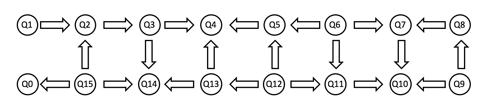
Figure 3. Schematic topology IBMQX5, taken from [30]. Directional arrows indicate the possibility of entanglement. For example, we could perform an operation (in QASM)but not surgery . To do this, the compiler translates instruction into equivalent gates, which are executed in the topology and set of gates.
C. ProjectQ
ProjectQ — это программная среда с открытым исходным кодом для квантовых вычислений с возможностью подключения к квантовым бэкендам IBM, высокопроизводительным квантовым компьютерным симулятором и несколькими библиотечными плагинами. Первый релиз ProjectQ был разработан Thomas Häner и Damien S. Steiger в группе Matthias Troyer в ETH Zurich, и с тех пор он набрал больше участников.
a. Требования и установка
Для установки ProjectQ требуется текущая версия Python (2.7 или 3.4+). Документация содержит подробную информацию об установке для каждой операционной системы. В нашей среде рекомендуется установка через :
python −m pip install −−user projectqдля успешной установки программного обеспечения (как пользователя). Для установки из исходного кода мы можем набрать следующее в командной строке:
git clone https://github.com/ProjectQ−Framework/ProjectQ
cd projectq
python −m pip install −−user
Как и в предыдущих программах, этот метод рекомендуется для пользователей, которые хотят внести свой вклад в исходный код. Инструкции по этому поводу смотрите в руководстве по вкладам на странице ProjectQ GitHub.
b. Документация и учебные материалы
ProjectQ имеет очень хорошую документацию по установке. Однако выделим, что оставшаяся часть документации немного скудна. В онлайн-учебном пособии представлены инструкции по базовому синтаксису и примерам квантовых программ (случайные числа, телепортация и алгоритм разложения Шора). Остальная часть — это документация/ссылка на код с информацией о структуре кода и каждом дополнительном модуле, включая функции и классы. Документы [18, 19] являются хорошими ссылками и источниками, но более вероятно, что онлайн-документация будет более актуальной.
c. Синтаксис
Синтаксис ProjectQ прост и практичен, хотя для этого нужно привыкнуть. Для ProjectQ нет языка квантового ассемблера (поскольку нет квантового бэкенда ProjectQ), но используется классический язык — своего рода гибридный классический/квантовый язык. Чтобы разъяснить, пример программы для создания случайного бита показан ниже:
# random number generator circuit in ProjectQfrom projectq import MainEngine
import projectq.ops as ops
eng = MainEngine()
qbits = eng.allocate_qureg(1)
    ops.H | qbits[0]
ops.Measure | qbits[0]
    eng.flush()
print(int(qbits[0]))
Листинг 6. Код ProjectQ для генератора случайных чисел.
В строке 2 импортируется необходимый модуль для создания квантовой схемы, а в строке 3 импортируются операции с гейтом. В строке 5 выделяется память и создаем движок (engine) , а в строке 6 мы выделяем один кубитный регистр. В строках 8 и 9 приводятся инструкции схемы: сначала действуем гейтом Адамара на кубит в регистре с индексом 0, затем измеряем этот кубит. Здесь «квантовый синтаксис» появляется на классически написанном языке. Общая формулировка — с вертикальной линией между двумя похожими на обозначения Дирака, , например. Затем мы сбрасываем движок, отправляя его на бэкэнд и обеспечивая его оценку/имитацию. В отличие от pyQuil и QISKit, в ProjectQ при измерении не указывается классический регистр. Вместо этого, когда мы измеряем в строке 9, мы получаем его значение, преобразовывая его в , когда выводим его в строке 12.
d. Квантовый язык
Как уже упоминалось, ProjectQ не имеет собственного специализированного квантового языка. Если вы используете ProjectQ совместно с бэкендом от IBM, код в конечном итоге будет преобразован в OpenQASM: язык квантового ассемблера IBM.
e. Квантовое аппаратное оборудование
ProjectQ не имеет собственного специализированного квантового компьютера. Тем не менее, каждый может использовать квантовые ресурсы IBM при использовании ProjectQ.
f. Симулятор
ProjectQ предоставляется с быстродействующим симулятором, написанным на C++, который будет установлен по умолчанию, если не возникнет ошибка, иначе будет установлен более медленный симулятор на Python. Кроме того, ProjectQ включает в себя для эффективного моделирования групповых схем (stabilizer circuits), т. е. схем, которые состоят из гейтов нормализатора группы Паули, которые могут быть получены из гейта Адамара, CNOT и фазового гейта [26]. Этот симулятор способен обрабатывать тысячи кубитов, чтобы проверить, например, схемы сумматора гейта Тоффоли, для конкретных данных. Однако групповые схемы не являются универсальными, поэтому наш тест и тестирование фокусируется на .
ProjectQ технически сложный и быстродействующий. На компьютере автора [23]() (отметим, что максимальное количество кубитов ограничено локальной памятью пользователя), он может обрабатывать схемы с 26 кубитами и глубиной 5 в минуту, а схемы с 28 кубитами и глубиной 20 — чуть меньше десяти минут. Полную информацию смотрите в разделе [III D]() и на Фигуре 6.
h. ProjectQ в других платформах
ProjectQ является хорошо проверенным, надежным кодом и используется для других платформ, упомянутых в этой статье. В частности, pyQuil содержит код ProjectQ [27], а ядра симулятора Microsoft QDK разработаны Thomas Häner и Damian Steiger из ETH Zurich [28], оригинальными авторами проекта. (Обратите внимание, что это не обязательно означает, что симулятор QDK достигает производительности симулятора ProjectQ C++, так как обернутый код может снизить производительность.)
D. Quantum Development Kit
В отличие от технологии сверхпроводящих кубитов Rigetti и IBM, Microsoft делает ставку на топологические кубиты на основе майорановских фермионов. Эти частицы были недавно обнаружены [29] и обеспечивают длительное время когерентности и другие требуемые свойства, но функционального квантового компьютера, использующего топологические кубиты, в настоящее время не существует. Таким образом, у Microsoft в настоящее время нет устройства, с которым пользователи могут подключаться через комплект Quantum Development Kit (QDK), самую молодую из четырех платформ, представленных в этой статье. Несмотря на это, QDK имеет новый «квантово-ориентированный» язык под названием Q#, который имеет высокую степень интеграции с Visual Studio и Visual Studio Code и может локально имитировать квантовые схемы до 30 кубитов. Это предварительное программное обеспечение было впервые дебютировано в январе 2018 года и, несмотря на все это находится в альфа-тестировании, с доступностью на MacOS, Windows и Linux.
a. Требования и установка
Несмотря на то, что в документации Visual Studio Code указана как дополнительная, установка настоятельно рекомендуется для всех платформ. (В этой статье мы используем только VS Code, но Visual Studio также является особой средой. Мы по-прежнему платформенно-независимо относимся к тому, что лучше, и нам предпочтительно использовать VS Code.) Как только это будет сделано, текущую версию QDK можно установить, введя следующее в командной строке Bash:
dotnet new −i "Microsoft.Quantum.ProjectTemplates::0.2 −*"Чтобы получить примеры кода и библиотеки QDK из репозитория GitHub (настоятельно рекомендуется всем и особенно тем, кто может внести свой вклад в QDK), можно дополнительно набрать:
git clone https://github.com/Microsoft/Quantum.git
cd Quantum
code
b. Документация и учебные материалы
Вышеприведенные примеры кода и библиотеки — отличный способ изучить язык Q#, а онлайн-документация содержит информацию о проверке успешной установки, запуске первой квантовой программы, квантового симулятора, стандартных библиотек Q# и языка программирования. Эта документация подробна и содержит большой объем информации; читатель может сам решить, является ли это плюсом или минусом.
c. Синтаксис
Синтаксис Q# совершенно отличается от предыдущих трех языков. Он очень похож на C#: более подробный, чем Python, и может иметь более крутую кривую обучения для тех, кто не знаком с C#. Ниже показана такая же схема генераторов случайных чисел, что и для всех языков:
// random number generator circuit in QDK
operation random (count: Int, initial: Result) : (Int, Int)
{
    body
    {
        mutable numOnes = 0;
        using ( qubits = Qubit[1])
        {
            for (test in1..count)
            {
                Set(initial, qubits[0]);
                H(qubits[0]);
                let res = M(qubits[0]);
                 // count the number of ones
                if (res == One)
                {
                   set numOnes = numOnes + 1;
                }
            }
            Set(Zero, qubits[0]);
        }
        // returnstatisticsreturn (count − numOnes, numOnes);
    }
}
Листинг 7. Код Q# для генератора случайных чисел.
Использование скобок и ключевых слов может, возможно, сделать этот язык немного более сложным для новичков при изучении/чтении, но по своей сути код выполняет ту же схему, что и предыдущие три примера. Для краткости мы опустим анализ кода. Заметим, однако, что это один из трех файлов, необходимых для запуска этого кода. Вышеуказанное — это файл для языка Q#, и нам также необходим файл для запуска кода, а также , содержащий метаданные. В общем, этот пример насчитывает около 65 строк кода. Поскольку этот пример можно найти в онлайн-документации, мы эти программы добавляются, но тем не менее заинтересованный читатель направляется к учебному пособию «Quickstart» в документации.
Автор хотел бы отметить, что QDK стремится к высокоуровневому языку, который абстрагируется от аппаратного обеспечения и облегчает пользователям программирование квантовых компьютеров. Как аналог, при составлении сложения на классическом компьютере не выделяется схема сумматора — это выполняется в высокоуровневой структуре , и программное обеспечение компилирует это на аппаратный уровень. Поскольку QDK ориентирован на разработку таких стандартов, что измерение легкости написания кода на основе простых примеров, таких как генератор случайных чисел и схема телепортации (смотрите Приложение C, может не оправдать общий синтаксис языка и возможности платформы, но тем не менее эти программы, имеющие определенную степень согласованности в нашем анализе, добавлены.
d. Квантовый язык / аппаратное обеспечение
Как уже упоминалось, QDK не имеет возможности подключаться к реальному квантовому компьютеру и не имеет специального языка квантового ассемблера. Однако язык Q# можно считать гибридным классическим/квантовым языком.
e. Симулятор
На локальном компьютере пользователя набор QDK включает в себя квантовый симулятор, который может запускать схемы до 30 кубитов. Как упоминалось выше, ядро для симулятора QDK было написано разработчиками ProjectQ, поэтому можно ожидать, что производительность будет аналогична производительности симулятора ProjectQ. (Смотрите Раздел III D.) Благодаря платной подписке на облако Azure можно получить доступ к высокопроизводительным вычислениям, которые позволяют моделировать более 40 кубитов. Однако в документации QDK в настоящее время мало инструкций о том, как это сделать.
Кроме того, QDK обеспечивает симулятор диагностики (trace simulator), которая очень эффективен для отладки классического кода, который является частью квантовой программы, а также оценки ресурсов, необходимых для запуска данного экземпляра квантовой программы на квантовом компьютере. Симулятор диагностики позволяет использовать различные показатели производительности для квантовых алгоритмов, содержащих тысячи кубитов. Схемы такого размера возможны, потому что симулятор диагностики выполняет квантовую программу без фактического моделирования состояния квантового компьютера. Рассматривается широкий спектр оценки ресурсов, включая подсчеты для гейта Клиффорда, Т-образного гейта, произвольно заданных квантовых операций и т. д. Он также позволяет определять глубину схемы на основе заданных длительностей гейтов. Полную информацию о симуляторе диагностики можно найти в онлайн-документации QDK.
Iii. Comparison
Later in this section, when the basics of each platform were considered, we will compare each of the additional characteristics, including support at the level of libraries, quantum equipment, and the quantum compiler. We will also list some noteworthy and useful features of each platform.
A. Library support
The term “support at the library level” is used to refer to examples of quantum algorithms (in training programs or documentation) or a specific function for a quantum algorithm (for example, ). We have already touched on some of them in the previous section. A more detailed table showing library level support for the four software platforms is shown in Figure 4.
Note that any algorithm, of course, can be implemented on any of these platforms. Here we will highlight the existing functionality that may be useful for users who are new to this field or even experienced, so as not to program everything themselves.
As can be seen from the table, pyQuil, QISKit and QDK have relatively large library support. ProjectQ contains FermiLib, FermiLib plugins, and it is compatible with OpenFermion, which are open source projects for quantum modeling algorithms. All the examples that work with these projects naturally work with ProjectQ. Microsoft QDK differs in the number of built-in functions that perform these algorithms automatically, without the need to explicitly program a quantum circuit. In particular, the QDK library offers a detailed iterative assessment phase, an important procedure in many algorithms that can be easily implemented in QDK without sacrificing adaptation. QISKit is distinguished by a large number of educational materials on a wide range of topics from fundamental quantum algorithms to instructive quantum games.
B. Quantum hardware
In this section, we will discuss only pyQuil and QISKit, since these are the only platforms with their own quantum hardware. Qubit is an important characteristic in quantum computers, but no less important - if not more important - the “quality of qubit”. By this is meant the coherence time (how long the qubits live until destruction in bits), the time to apply the gate, the gate error rate, and the topology / connectivity of the qubits. Ideally, one would have infinite coherence time, zero gate time, zero error rate, and many-to-many connectedness. In the following paragraphs, we describe some of the characteristics of IBMQX5 and Agave, the two largest publicly available quantum computers. For details, see the online documentation for each platform.
a. IBMQX5
IBMQX5 is a 16-qubit superconducting quantum computer with connected nearest neighbors (see Figure 3). The minimum coherence time (T2) is microseconds on the 0th qubit, and the maximum microseconds on the 15th qubit. A single-qubit gate requires 80 nanoseconds per execution and plus 10 nanoseconds per depreciation after each pulse. Gates it takes about two to four times longer, starting at 170 nanoseconds for up to 348 nanoseconds for . The playback quality of a single-qubit gate is very good with an accuracy of more than 99.5% for all qubits (accuracy = 1 is an error). Multi-qubit accuracy is higher than 94.9% for all pairs of qubits in the topology. The largest read error is quite large at about 12.4%, with an average of about 6%. These statistics were obtained from [30].
Finally, we mention that to use any available IBM quantum computer, the user sends his or her work to a queue that determines when the task starts. This is different from using Agave from Rigetti, in which users must first request access through an online form, and then schedule time to access the device to run tasks. According to the author’s experience, this is done via email and the staff is very responsive.
b. Agave
The Agave quantum computer consists of 8 superconducting transmon (transmon) qubits with a fixed capacitive coupling and connectivity shown in Figure 2. The minimum coherence time (T2) is 9.2 microseconds on the 1st qubit, and the maximum is 15.52 microseconds for 2 th Qubit The implementation time on the gate Controlled-ranges from 118 to 195 nanoseconds. The accuracy of a single-qubit gate averages 96.2% (again, accuracy = 1 is an error) and at least 93.2%. The accuracy of a multi-qubit gate averages 87% for all pairs of qubit-qubit in the topology. Read errors are unknown. These statistics can be found in the online documentation or via pyQuil.
| Algorithm | pyQuil | QISKit | ProjectQ | QDK |
|---|---|---|---|---|
| Random number generator | (T) | (T) | (T) | (T) |
| Teleportation | (T) | (T) | (T) | (T) |
| Swap test | (T) | |||
| Deutsch-Jozsa | (T) | (T) | (T) | |
| Grover's Algorithm | (T) | (T) | (T) | (B) |
| Quantum Fourier Transform | (T) | (T) | (B) | (B) |
| Shor's Algorithm | (T) | (D) | ||
| Bernstein vazirani | (T) | (T) | (T) | |
| Phase Estimation | (T) | (T) | (B) | |
| Optimization / QAOA | (T) | (T) | ||
| Simon's Algorithm | (T) | (T) | ||
| Variational quantum eigensolver | (T) | (T) | (P) | |
| Amplitude amplification | (T) | (B) | ||
| Quantum Walk | (T) | |||
| Ising solver | (T) | (T) | ||
| Quantum Gradient Descent | (T) | |||
| Five Qubit Code | (B) | |||
| Repetition code | (T) | |||
| Steane code | (B) | |||
| Draper adder | (T) | (D) | ||
| Beauregard adder | (T) | (D) | ||
| Arithmetic | (B) | (D) | ||
| Fermion transforms | (T) | (T) | (P) | |
| Trotter Simulation | (D) | |||
| Electronic Structure (FCI, MP2, HF, etc.) | (P) | |||
| Process tomography | (T) | (T) | (D) | |
| Meyer-penny game | (D) | |||
| Vaidman Detection Test | (T) | |||
| Battleships game | (T) | |||
| Emoji game | (T) | |||
| Counterfeit Coin Game | (T) |
Figure 4. A table showing support at the library level for each of the four software platforms. By “support at the library level” is meant an educational material or program (T), an example in the documentation (D), a built-in function (B) for a language or a supported plug-in library (P).
C. Quantum Compilers
Platforms that provide connectivity to real quantum devices must necessarily have a means of translating this scheme into operations that a computer can understand. This process is known as translation or more detailed translation of a quantum scheme / quantum translation . Each computer has a basic set of gates and a certain connectedness - the task of the compiler is to obtain a given scheme and return an equivalent scheme obeying the requirements of the basis and the requirements for connectedness. In this section, we will discuss only QISKit and Rigetti, since these are platforms with real quantum computers.
The basis of IBMQX5 are , , and where

notice, that equivalent to changing the gate to the global phase as well and - sequence of gates and impulses changes

with turn gates being standard.

Where and - ordinary Pauli matrices. On IBM Quantum Computersis a “virtual gate”, which means that nothing physically happens to the qubit. Instead, since qubits naturally rotate around the axismaking rotation it just comes down to changing the clock or frames of the internal (classic) software that tracks the qubit.
The IBMQX5 topology is shown in Figure 3. This connectivity determines which qubits can be initially performed. where matrix representation is given by the formula

Note that execution is possible. between any qubits in QISKit, but when the program is compiled to the hardware level, the QISKit compiler converts this into a sequence of CNOT gates satisfying the connectivity. The QISKit compiler allows you to specify an arbitrary set of basic gates and topology, as well as provide a set of parameters, such as noise.
For 8-qubit Agave Rigetti processor base blocks for , and controlled-. Single-qubit turn gates, as above, and two qubits Controlled- () are given by the formula

The Agave topology is shown in Figure 2. Like QISKit, the pyQuil compiler also allows you to specify the target instruction set architecture (set of basic gates and computer topology).
An example of the same quantum scheme compiled by both platforms is shown in Figure 5. Here, using pyQuil, the program is broadcast to the characteristics of Agave, and with QISKit - IBMQX5. As you can see, QISKit creates a longer schema (i.e., has a greater depth) than pyQuil. It is impractical to argue that one of the compilers is superior because of this example. Schemes in a language that IBMQX5 understands more naturally will result in a shorter scheme than those on pyQuil, and vice versa. It is known that any quantum scheme (unitary matrix) can be decomposed into a sequence of one- and two-qubit gates (see, for example, [32]), but in general, a significant number of gates are needed for this. Now of considerable interest is the question [46], which consists in finding the optimal compiler for a given topology.

Figure 5. An example of a quantum scheme (top left) compiled by pyQuil for an 8-qubit Agave processor from Rigetti (top right) and the same scheme compiled by QISKit for IBM IBM QX5 computer with 16 qubits. The qubits used in Agave are 0, 1, and 2 (see Figure 2), and the qubits used in IBMQX5 are 0, 1, and 2. Note that no compiler can directly implement Hadamard gatebut produces them through a sequence of turn gates and . Gate can be implemented on IBMQX5, but not on Agave - here pyQuil should express with the help of gates Controlled-and rotations. These schemes were made using ProjectQ.
D. Simulator performance
Not all software platforms provide communication with real quantum computers, but any expedient program includes a quantum circuit simulator. This is a program that runs on a classical processor that simulates (that is, simulates) the process of changing a quantum computer. As in the case of quantum equipment, it is important to consider not only the number of qubits that the simulator can process, but also how quickly it can process them, in addition to other parameters, such as adding noise to simulate quantum computers, etc. section, we estimate the performance of the local QISKit vector state simulator and the local simulator written in C ++, ProjectQ using the program specified in Appendix B. First, we mention the performance of the simulator QVM pyQuil.
a. pyQuil
The Rigetti simulator, called Quantum Virtual Machine (QVM), does not run on the user's local computer, but rather due to the use of computing resources in the cloud. As already mentioned, this requires an API key. Most API keys give access to 30 qubits initially, and access to more can be requested. The author can simulate a 16-qubit scheme and a depth of 10 on average in 2.61 seconds. The circuit size of 23 qubits and a depth of 10 was modeled in 56.33 seconds, but no larger circuits could be modeled because QVM exits after one minute of calculation using the current API access key. Due to limited time and because QVM does not start on the user's local computer, we do not check the performance of QVM the same
QVM contains complex and flexible noise models for emulating the work process of a real quantum computer. This is the key to the development of shallow-depth algorithms on quantum computers in the near future, as well as for the theoretical evaluation of the results of calculations for a particular quantum chip. Users can define arbitrary noise models for testing programs, in particular, identify noisy gates, add decoherence noise, and read model noise. See the Noise and Quantum Computation section of the pyQuil documentation for details and useful sample programs .
b. QISKit
QISKit has several quantum simulators available as a backend: , , , and . A distinctive feature of these simulators is the principle of modeling quantum schemes. The unitary simulator implements the basic (unitary) matrix multiplication and is sharply limited to the operational memory. A full unitary matrix is not stored in the vector state simulator, but only the state vector and one / several qubit gate are loaded. Both methods are discussed in [33], and [34-36] contain detailed information about other methods. Like the reasoning about in ProjectQ, able to effectively imitate group circuits (stabilizer circuits), which are not universal.
Using a local unitary simulator, the scheme for 10 qubits and a depth of 10 is modeled in 23.55 seconds. Adding another qubit increases the time by about ten times - 239.97 seconds, and with 12 qubits, the simulator exceeds the waiting time after 1000 seconds (about 17 minutes). This simulator quickly achieves long simulation times and memory limitations, since for qubits should be kept in memory unitary size matrix .
The simulator of the vector state considerably exceeds the unitary simulator. We can simulate a circuit of 25 qubits in just three minutes. All schemes up to 20 qubit with a depth of thirty are simulated in less than five seconds. See Figures 6 and 7 for details.
with. ProjectQ
ProjectQ comes with a high-performance C ++ simulator that showed the best results in our private testing. The maximum size scheme, which we were able to successfully imitate, was 28 qubits, which took a little less than ten minutes (569.71 seconds) with a scheme depth of 20. Implementation details, see [18]. For full performance and testing, see Figures 6 and 7.

Figure 6. Characteristics of the local QISKit vector state simulator (above) and the ProjectQ simulator in C ++ (below), showing the execution time in seconds for a given number of qubits (horizontal axis) and the depth of the circuit (vertical axis). Dark green color indicates the shortest time, and bright yellow color indicates the longest time (color scales do not match for both graphs). For more information about testing, see Appendix ** B **.

Figure 7. The circuit used to test the ProjectQ simulator in C ++ and the local QISKit vector state simulator is shown here on four qubits. In actual testing, a combination of Hadamard's gate, then a sequence of gate CNOT, determined by one level in the scheme. This combination is repeated until the desired depth is reached. This image was created using ProjectQ.
E. Features
A good feature of pyQuil is Grove, located in a separate repository on GitHub, which can be installed with tutorials and examples of algorithms using pyQuil. Rigetti also creates a solid user community, an example of which is their dedicated Slack channel for Rigetti Forest. Also useful is the Quil compiler and the ability to compile for any given set of architecture instructions (topology and base gates). Finally, pyQuil is compatible with OpenFermion [37], open source Python for compiling and analyzing quantum algorithms for modeling fermion systems, including quantum chemistry.
QISKit is also available to users with experience in JavaScript and Swift. For beginners, the Python language is a very good starting programming language because of its easy and intuitive syntax. Like Grove, QISKit also contains a special repository of example algorithms and guidelines. In addition, the ACQUA library in QISKit contains numerous algorithms for quantum chemistry and artificial intelligence. This library can be run via a graphical user interface or from the command line interface. IBM is unmatched to build an active community of students and researchers using their platform. The company boasts more than 3 million remote launches of cloud quantum computing resources using QISKit, which is managed by more than 80,000 registered users, and more than 60 scientific publications were written using technology from IBM [31]. QISKit also has a dedicated channel on Slack with the ability to view a job in a queue, which is a useful feature for determining how long a sent job will run. In addition, the newest version of QISKit contains an inbuilt schematic drawer.
Likewise, ProjectQ contains a schematic drawer. By adding just a few lines of code to the program, you can create code in TikZ to create high-quality images in. All quantum circuits in this article were made using ProjectQ. The local simulator ProjectQ is also an excellent feature, as it has a very high performance. Although ProjectQ does not have its own quantum hardware, users can connect to quantum hardware from IBM. In addition, ProjectQ has several libraries, including OpenFermion, as mentioned above.
QDK was available exclusively on Windows until February 2018, he received support for macOS and Linux. The ability to implement quantum algorithms without explicit programming of the circuit is a nice feature of QDK, and there are many good guides in the documentation and examples folder for quantum algorithms. It is also noteworthy that Q # provides automatic generation functions for, for example, a coupled or controlled version of a quantum operation. In a more general sense, QDK identifies and offers important tools for developing a productive quantum algorithm, including testing quantum programs, estimating resource requirements, programming on various quantum computing models focused on different hardware, and ensuring the correctness of quantum programs at the compilation stage.
Iv. Discussion and conclusions
At this stage, it is assumed that the reader will have enough information and understanding to make an informed decision about which platform (s) for quantum software is appropriate for him. The next step is to start reading the documentation on the platform, install it, and start coding. In a short time, you can run algorithms on real quantum devices and start researching / developing algorithms in your area.
For those who have not yet decided, the following subjective recommendations are offered:
- For those whose primary purpose is to use quantum computers, QISKit (or ProjectQ) or pyQuil is the obvious choice.
- For those new to quantum computing, QISKit, pyQuil, or QDK is a good choice.
- For those who have little programming experience, one of the Python platforms is a good choice.
- For those who are familiar with or prefer C / C # style syntax, QDK is a good choice.
- For those who want to develop prototype and test algorithms, ProjectQ is a good choice.
- For those who want to use hybrid quantum-classical algorithms, pyQuil is an excellent choice for dedicated planned use of hardware time.
- For those interested in the continuous variables in quantum computing, see Strawberry Fields in Appendix A .
Again, these are just recommendations, and the reader is encouraged to make a choice. All platforms are significant advances in quantum computing and are excellent utilities for students and researchers in programming real quantum computers. As a final note, we note that developed additional software packages, some of which are referred to in Annex A .
Список литературы
- Bernhard Ömer, A procedural formalism for quantum computing, Master’s thesis, Department of Theoretical Physics, Technical University of Vienna, 1998.
- S. Bettelli, L. Serafini, T. Calarco, Toward an architecture for quantum programming, Eur. Phys. J. D, Vol. 25, No. 2, pp. 181-200 (2003).
- Peter Selinger (2004), A brief survey of quantum programming languages, in: Kameyama Y., Stuckey P.J. (eds) Functional and Logic Programming. FLOPS 2004. Lecture Notes in Computer Science, vol 2998. Springer, Berlin, Heidelberg.
- Benjamin P. Lanyon, James D. Whitfield, Geoff G. Gillet, Michael E. Goggin, Marcelo P. Almeida, Ivan Kassal, Jacob D. Biamonte, Masoud Mohseni, Ben J. Powell, Marco Barbieri, Alaґn Aspuru-Guzik, Andrew G. White, Towards quantum chemistry on a quantum computer, Nature Chemistry 2, pages 106-111 (2010), doi:10.1038/nchem.483.
- Jonathan Olson, Yudong Cao, Jonathan Romero, Peter Johnson, Pierre-Luc Dallaire-Demers, Nicolas Sawaya, Prineha Narang, Ian Kivlichan, Michael Wasielewski, Alaґn Aspuru-Guzik, Quantum information and computation for chemistry, NSF Workshop Report, 2017.
- Jacob Biamonte, Peter Wittek, Nicola Pancotti, Patrick Rebentrost, Nathan Wiebe, Seth Lloyd, Quantum machine learning, Nature volume 549, pages 195-202 (14 September 2017).
- Seth Lloyd, Masoud Mohseni, Patrick Rebentrost, Quantum principal component analysis, Nature Physics volume 10, pages 631-633 (2014).
- Vadim N. Smelyanskiy, Davide Venturelli, Alejandro Perdomo-Ortiz, Sergey Knysh, and Mark I. Dykman, Quantum annealing via environment-mediated quantum diffusion, Phys. Rev. Lett. 118, 066802, 2017.
- Patrick Rebentrost, Brajesh Gupt, Thomas R. Bromley, Quantum computational finance: Monte Carlo pricing of financial derivatives, arXiv preprint (arXiv:1805.00109v1), 2018.
- I. M. Georgescu, S. Ashhab, Franco Nori, Quantum simulation, Rev. Mod. Phys. 86, 154 (2014), DOI: 10.1103/RevModPhys.86.153.
- E. F. Dumitrescu, A. J. McCaskey, G. Hagen, G. R. Jansen, T. D. Morris, T. Papenbrock, R. C. Pooser, D. J. Dean, P. Lougovski, Cloud quantum computing of an atomic nucleus, Phys. Rev. Lett. 120, 210501 (2018), DOI: 10.1103/PhysRevLett.120.210501.
- Lukasz Cincio, Yigit Subasi, Andrew T. Sornborger, and Patrick J. Coles, Learning the quantum algorithm for state overlap, arXiv preprint (arXiv:1803.04114v1), 2018
- Patrick J. Coles, Stephan Eidenbenz, Scott Pakin, et al., Quantum algorithm implementations for beginners, arXiv preprint (arXiv:1804.03719v1), 2018.
- Mark Fingerhuth, Open-Source Quantum Software Projects, accessed May 12, 2018.
- Quantiki: List of QC Simulators, accessed May 12, 2018
- R. Smith, M. J. Curtis and W. J. Zeng, A practical quantum instruction set architecture, 2016.
- QISKit, originally authored by Luciano Bello, Jim Challenger, Andrew Cross, Ismael Faro, Jay Gambetta, Juan Gomez, Ali Javadi-Abhari, Paco Martin, Diego Moreda, Jesus Perez, Erick Winston, and Chris Wood, https://github.com/QISKit/qiskit-sdk-py.
- Damian S. Steiger, Thomas Häner, and Matthias Troyer ProjectQ: An open source software framework for quantum computing, 2016.
- Thomas Häner, Damian S. Steiger, Krysta M. Svore, and Matthias Troyer A software methodology for compiling quantum programs, 2016.
- The Quantum Development Kit by Microsoft, homepage: https://www.microsoft.com/en — us/quantum/development-kit, github: https://github.com/Microsoft/Quantum.
- Michael A. Nielsen and Isaac L. Chuang, Quantum Computation and Quantum Information 10th Anniversary Edition, Cambridge University Press, 2011.
- Doug Finke, Education, Quantum Computing Report, https://quantumcomputingreport.com/resources/education/, accessed May 26, 2018.
- All code in this paper was run and tested on a Dell XPS 13 Developer Edition laptop running 64 bit Ubuntu 16.04 LTS with 8 GB RAM and an Intel Core i7-8550U CPU at 1.80 GHz. Programs were run primarily from the command line but the Python developer environment Spyder was also used for Python programs and Visual Studio Code was used for C# (Q#) programs.
- Forest: An API for quantum computing in the cloud, https://www.rigetti.com/index.php/forest, accessed May 14, 2018.
- Andrew W. Cross, Lev S. Bishop, John A. Smolin, Jay M. Gambetta, Open quantum assembly language, 2017.
- Scott Aaronson, Daniel Gottesman, Improved Simulation of Stabilizer Circuits, Phys. Rev. A 70, 052328, 2004.
- pyQuil Lisence, github.com/rigetticomputing/pyquil/blob/master/LICENSE#L204, accessed June 7, 2018.
- Microsoft Quantum Development Kit License, marketplace.visualstudio.com/items/quantum.DevKit/license, accessed June 7, 2018.
- Hao Zhang, Chun-Xiao Liu, Sasa Gazibegovic, et al. Quantized Majorana conductance, Nature 556, 74-79 (05 April 2018).
- 16-qubit backend: IBM QX team, “ibmqx5 backend specification V1.1.0,” (2018). Retrieved from https://ibm.biz/qiskit-ibmqx5 and https://quantumexperience.ng.bluemix.net/qx/devices on May 23, 2018.
- Talia Gershon, Celebrating the IBM Q Experience Community and Their Research, March 8, 2018.
- M. Reck, A. Zeilinger, H.J. Bernstein, and P. Bertani, Experimental realization of any discrete unitary operator, Physical Review Letters, 73, p. 58, 1994.
- Ryan LaRose, Distributed memory techniques for classical simulation of quantum circuits, arXiv preprint (arXiv:1801.01037v1), 2018.
- Thomas Haner, Damian S. Steiger, 0.5 petabyte simulation of a 45-qubit quantum circuit, arXiv preprint (arXiv:1704.01127v2), September 18, 2017.
- Jianxin Chen, Fang Zhang, Cupjin Huang, Michael Newman, Yaoyun Shi, Classical simulation of intermediate-size quantum circuits, arXiv preprint (arXiv:1805.01450v2), 2018.
- Alwin Zulehner, Robert Wille, Advanced simulation of quantum computations, arXiv preprint (arXiv:1707.00865v2), November 7, 2017.
- Jarrod R. McClean, Ian D. Kivlichan, Kevin J. Sung, et al., OpenFermion: The electronic structure package for quantum computers, arXiv:1710.07629, 2017.
- Nathan Killoran, Josh Izaac, Nicols Quesada, Ville Bergholm, Matthew Amy, Christian Weedbrook, Strawberry Fields: A Software Platform for Photonic Quantum Computing, arXiv preprint (arXiv:1804.03159v1), 2018.
- IonQ website, https://ionq.co/, accessed June 15, 2018.
- D-Wave: The quantum computing company, https://www.dwavesys.com/home, accessed June 20, 2018.
- Вплоть до 4 июня 2018 года у Rigetti был 20-ти кубитный компьютер, который являлся общедоступным для использования. Согласно электронной почте от сотрудников службы поддержки, замена на 8-ми кубитный чип произошла «из-за ухудшения производительности». Неясно, является ли эта замена временной или 20-ти кубитный процессор будет удален навсегда (и, возможно, заменен новым чипом).
- Текущими членами IBMQ Network являются те, кто был объявлен в декабре 2017 года — JP Morgan Chase, Daimler, Samsung, Honda, Oak Ridge National Lab, — и другие, анонсированные в апреле 2018 года — Zapata Computing, Strangeworks, QxBranch, Quantum Benchmark, QC Ware, Q-CTRL, Cambridge Quantum Computing (CQC), и 1QBit. North Carolina State University является первым американским университетом, который будет членом IBM Q Hub, который также включает в себя University of Oxford и University of Melbourne. Полный и обновленный список смотрите в https://www.research.ibm.com/ibmq/network/.
- Действительно, все четыре из этих платформ в настоящее время являются альфа- или бета-программным обеспечением. При написании этой статьи были выпущены две новые версии QISKit, а также новая библиотека ACQUA для химии и искусственного интеллекта, и была выпущена новая версия pyQuil.
- Это обычный синтаксис pyQuil для импорта только используемых гейтов: например, . Автор предпочитает импортировать весь для операторной прозрачности и для сравнения с другими языками программирования, но обратите внимание, что предпочтительным методом разработчика является первый, который может незначительно помочь ускорить код и держать программы более опрятными.
- Мы могли бы просто объявить один кубит и один классический бит для этой программы вместо того, чтобы иметь регистр и ссылаться на (ку)биты по индексу. Однако, для более крупных схем обычно проще указывать регистры и ссылаться на (ку)биты по индексу, чем на отдельные названия, поэтому мы придерживаемся этой практики здесь.
- Конкурс от IBM, завершившийся 31 мая 2018 года, «задача квантового разработчика» заключается в написании лучшего кода компилятора в Python или Cython, которому подают на вход квантовую схему и получают оптимальную схему для данной топологии.
A. Другие программные платформы
Как уже упоминалось в основном тексте, было бы нецелесообразно включать анализ всех программных платформ или компаний с квантовыми вычислениями. Обновленный и текущий список смотрите на странице Players в отчете Quantum Computing Report [22]. Наши выбранные варианты в этой статье во многом определялись возможностью обычных пользователей подключиться к реальным квантовым устройствам и использовать их, а также неизбежными личными факторами, такими как опыт автора. Наше опущение программного обеспечения/компаний не является заявлением об их неработоспособности — здесь кратко упомминаются некоторые.
a. Strawberry Fields
Разработанный стартапом Xanadu, основанным в Торонто, Strawberry Fields представляет собой полноценную библиотеку для Python по проектированию, моделированию и оптимизации квантовых оптических схем [38]. Xanadu разрабатывает фотонные квантовые компьютеры с непрерывными переменными или «qumodes» (в отличие от дискретных переменных кубитов), и, хотя компания еще не объявила о выпуске доступной квантовой микросхемы для обычных пользователей, она может стать доступна в ближайшем будущем. Strawberry Fields имеет встроенные симуляторы с использованием Numpy и TensorFlow, а также язык квантового программирования Blackbird. Есть возможость загрузить исходный код с GitHub, и, например, найти учебные пособия для квантовой телепортации, выборки бозонов и машинного обучения. Кроме того, сайт Xanadu https://www.xanadu.ai/ содержит интерактивную квантовую схему, в которой пользователи могут перетаскивать гейты или выбирать из библиотеки примерные алгоритмы.
b. IonQ
IonQ — новая стартап-компания, находящаяся в College Park штата Мэриленд, и возглавляемая исследователями из Университета Мэриленда и Университета Дьюка. IonQ использует метод захваченных ионов для архитектуры квантовых вычислений, который обладает некоторыми очень подходящими свойствами. Используя ядерный спин Yb в виде кубита, IonQ достигла T2 (декогеренции) равной 15-ти минутам, в то время как более распространено время T2 равной 1 секунде. Кроме того, время релаксации T1 (время релаксации возбуждения) составляет порядка 20 000 лет, а ошибки однокубитового квантового гейта составляют около с использованием рамановских переходов. Для схем малого размера, связанность многие-ко-многим доступна из-за широких диапазонов кулоновских взаимодействий между ионами, и можно «перебросить» кубиты в разные линейные массивы для достижения универсальной связи в больших схемах. Также были продемонстрированы более интересные эффекты, такие как нелокальная телепортация между кубитами посредством излучения фотонов.
Аппаратное обеспечение IonQ в настоящее время недоступно через программный интерфейс для обычных пользователей, но можно связаться с IonQ и запросить доступ. Экспериментаторы запускали различные алгоритмы от машинного обучения до теории игр. Чтобы узнать больше о компании, посетите их веб-сайт [39].
c. D-Wave Systems
D-Wave [40], возможно, является самой старой компанией с квантовыми вычислениями. D-Wave, основанная в 1999 году в Ванкувере, Канада, создает специальные типы адиабатических квантовых компьютеров, известных как квантовые отжиги, которые решают для основного состояния энергии модели Изинга поперечного поля
D-Wave выпустила несколько компьютеров, самый последний из которых — в 2048 кубитов, и имеет широкое программное обеспечение в Matlab, C/C++ и Python для их программирования. Поскольку эти квантовые компьютеры не работают на модели квантовых вычислений с гейтами/схемами, D-Wave не было включено в основную часть текста. Однако исключение D-Wave не дает точной картины текущего ландшафта квантовых вычислений.
B. Тестирование производительности симулятора
Ниже приведен список программ для тестирования производительности локального симулятора ProjectQ на C++. Эти тесты были выполнены на Dell XPS 13 Developer Edition с 64-разрядным Ubuntu 16.04 LTS с 8 ГБ оперативной памяти и процессором Intel Core i7-8550U на частоте 1,80 ГГц.
# ------------------------------------------------------------------------------# imports# ------------------------------------------------------------------------------from projectq import MainEngine
import projectq.ops as ops
from projectq.backends import Simulator
import sys
import time
# ------------------------------------------------------------------------------# number of qubits and depth# ------------------------------------------------------------------------------if len(sys.argv) > 1:
    n = int(sys.argv[1])
else:
    n = 16if len(sys.argv) > 1:
    depth = int(sys.argv[2])
else:
    depth = 10# ------------------------------------------------------------------------------# engine and qubit register# ------------------------------------------------------------------------------
eng = MainEngine(backend=Simulator(gate_fusion=True), engine_list=[])
qbits = eng.allocate_qureg(n)
# ------------------------------------------------------------------------------# circuit# ------------------------------------------------------------------------------# timing -- get the start time
start = time.time()
# random circuitfor level in range(depth):
    for q in qbits:
        ops.H | q
        ops.SqrtX | q
        if q != qbits[0]:
            ops.CNOT | (q, qbits[0])
# measurefor q in qbits:
    ops.Measure | q
# flush the engine
eng.flush()
# timing -- get the end time
runtime = time.time() - start
# print out the runtime
print(n, depth, runtime)
Схема, которая была выбрана случайным образом, показана на Фигуре 7. Отметим, что симулятор QISKit был протестирован на идентичной схеме — опустим код для краткости.
C. Пример программы: Схема телепортации
В этом разделе мы продемонстрируем программы для схемы квантовой телепортации на каждом из четырех языков для сравнения бок о бок. Заметим, что показанная программа QDK является одной из трех программ, необходимых для выполнения схемы, как обсуждалось в основной части. Схема телепортации является стандартной для квантовых вычислений и отправляет неизвестное состояние из одного кубита — обычно первый или верхний кубит в схеме, — другому — обычно последний или нижний кубит в схеме. Базовая информация об этом процессе может быть найдена в любом стандартном источнике о квантовых вычислений или квантовой механики. Эта квантовая схема более сложна, чем очень маленькие программы, показанные в основном тексте, и демонстрирует несколько более продвинутые функции каждого языка — например, выполнение условных операций.
Для полноты добавим схему, чтобы сделать ее более ясной, что делают программы. В отличие от основного текста это изображение было сделано с использованием нового рисователя схем, выпущенного в последней версии QISKit.

Фигура 8. Схема телепортации, созданная с помощью , добавденный в QISKit v0.5.4.
pyQuil
#!/usr/bin/env python3# -*- coding: utf-8 -*-# ==============================================================================# teleport.py## Teleportation circuit in pyQuil.# ==============================================================================# ------------------------------------------------------------------------------# imports# ------------------------------------------------------------------------------from pyquil.quil import Program
from pyquil import api
import pyquil.gates as gate
# ------------------------------------------------------------------------------# program and simulator# ------------------------------------------------------------------------------
qprog = Program()
qvm = api.QVMConnection()
# ------------------------------------------------------------------------------# teleportation circuit# ------------------------------------------------------------------------------# teleport |1> to qubit three
qprog += gates.X(0)
# main circuit
qprog += [gates.H(1),
          gates.CNOT(1, 2),
          gates.CNOT(0, 1),
          gates.H(0),
          gates.MEASURE(0, 0),
          gates.MEASURE(1, 1)]
# conditional operations
qprog.if_then(0, gates.Z(2))
qprog.if_then(1, gates.X(2))
# measure qubit three
qprog.measure(2, 2)
# ------------------------------------------------------------------------------# run the circuit and print the results# ------------------------------------------------------------------------------
print(qvm.run(qprog))
# optionally print the quil code
print(qprog)
QISKit
#!/usr/bin/env python3# -*- coding: utf-8 -*-# ==============================================================================# teleport.py## Teleportation circuit in QISKit.# ==============================================================================# ------------------------------------------------------------------------------# imports# ------------------------------------------------------------------------------from qiskit import QuantumRegister, ClassicalRegister, QuantumCircuit, execute
# ------------------------------------------------------------------------------# registers and quantum circuit# ------------------------------------------------------------------------------
qreg = QuantumRegister(3)
creg = ClassicalRegister(3)
qcircuit = QuantumCircuit(qreg, creg)
# ------------------------------------------------------------------------------# do the circuit# ------------------------------------------------------------------------------# teleport |1> to qubit three
qcircuit.x(qreg[0])
# main circuit
qcircuit.h(qreg[0])
qcircuit.cx(qreg[1], qreg[2])
qcircuit.cx(qreg[0], qreg[1])
qcircuit.h(qreg[0])
qcircuit.measure(qreg[0], creg[0])
qcircuit.measure(qreg[1], creg[1])
# conditional operations
qcircuit.z(qreg[2]).c_if(creg[0][0], 1)
qcircuit.x(qreg[2]).c_if(creg[1][0], 1)
# measure qubit three
qcircuit.measure(qreg[2], creg[2])
# ------------------------------------------------------------------------------# run the circuit and print the results# ------------------------------------------------------------------------------
result = execute(qcircuit, 'local_qasm_simulator').result()
counts = result.get_counts()
print(counts)
# optionally print the qasm code
print(qcircuit.qasm())
# optionally draw the circuitfrom qiskit.tools.visualization import circuit_drawer
circuit_drawer(qcircuit)
ProjectQ
#!/usr/bin/env python3# -*- coding: utf-8 -*-# ==============================================================================# teleport.py## Teleportation circuit in ProjectQ.# ==============================================================================# ------------------------------------------------------------------------------# imports# ------------------------------------------------------------------------------from projectq import MainEngine
from projectq.meta import Control
import projectq.ops as ops
# ------------------------------------------------------------------------------# engine and qubit register# ------------------------------------------------------------------------------# engine
eng = MainEngine()
# allocate qubit register
qbits = eng.allocate_qureg(3)
# ------------------------------------------------------------------------------# teleportation circuit# ------------------------------------------------------------------------------# teleport |1> to qubit three
ops.X | qbits[0]
# main circuit
ops.H | qbits[1]
ops.CNOT | (qbits[1], qbits[2])
ops.CNOT | (qbits[0], qbits[1])
ops.H | qbits[0]
ops.Measure | (qbits[0], qbits[1])
# conditional operationswith Control(eng, qbits[1]):
    ops.X | qbits[2]
with Control(eng, qbits[1]):
    ops.Z | qbits[2]
# measure qubit three
ops.Measure | qbits[2]
# ------------------------------------------------------------------------------# run the circuit and print the results# ------------------------------------------------------------------------------
eng.flush()
print("Measured:", int(qbits[2]))
Quantum Developer Kit
// =============================================================================// teleport.qs//// Teleportation circuit in QDK.// =============================================================================
operation Teleport(msg : Qubit, there : Qubit) : () {
    body {
        using (register = Qubit[1]) {
            // get auxiliary qubit to prepare for teleportation
            let here = register[0];
            // main circuit
            H(here);
            CNOT(here, there);
            CNOT(msg, here);
            H(msg);
            // conditional operationsif (M(msg) == One)  { Z(there); }
            if (M(here) == One) { X(there); }
            // reset the "here" qubit
            Reset(here);
        }
    }
}
operation TeleportClassicalMessage(message : Bool) : Bool {
    body {
        mutable measurement = false;
        using (register = Qubit[2]) {
            // two qubits
            let msg = register[0];
            let there = register[1];
            // encode message to sendif (message) { X(msg); }
            // do the teleportation
            Teleport(msg, there);
            // check what message was sentif (M(there) == One) { set measurement = true; }
            // reset all qubits
            ResetAll(register);
        }
        return measurement;
    }
}