Numerical solution of mathematical models of objects given by systems of differential equations
Introduction:
In mathematical modeling of a number of technical devices, systems of differential nonlinear equations are used. Such models are used not only in technology, they are used in economics, chemistry, biology, medicine, management.
The study of the functioning of such devices requires the solution of these systems of equations. Since the main part of such equations are nonlinear and non-stationary, it is often impossible to obtain their analytical solution.
There is a need to use numerical methods, the most famous of which is the Runge – Kutta method [1]. As for Python, in publications on numerical methods, for example [2,3], there are very few data on the use of Runge - Kutta, and on its modification - in general there is no Runge-Kutta-Fellberg method.
Currently, thanks to a simple interface, the most popular in Python is the odeint function from the scipy.integrate module. The second ode function from this module implements several methods, including the mentioned five-rank Runge-Kutta-Fellberg method, but due to its universality, it has limited speed.
The purpose of this publication is a comparative analysis of the listed tools for the numerical solution of systems of differential equations with a modified author under the Python method of Runge-Kutta-Fellberg. The publication also provides solutions for boundary value problems for systems of differential equations (SDEs).
Brief theoretical and actual data on the considered methods and software for the numerical solution of the CDS
Cauchy problem
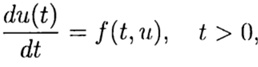
For a single nth order differential equation, the Cauchy problem is to find a function that satisfies the equality:
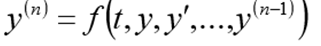
and initial conditions.

Before solving this problem, this problem must be rewritten as the following SDE
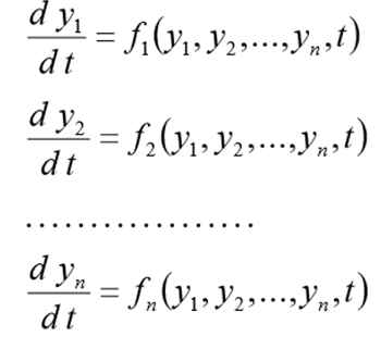 (1)
(1) with initial conditions.

Module scipy.integrate
The module has two functions ode () and odeint (), designed to solve systems of ordinary differential equations (ODE) of the first order with initial conditions at one point (the Cauchy problem). The ode () function is more versatile, and the odeint () function (ODE integrator) has a simpler interface and solves most problems well.
Odeint () function
The odeint () function has three required arguments and many options. It has the following format: odeint (func, y0, t [, args = (), ...]) The argument func is the name of the Python function of two variables, the first of which is the list y = [y1, y2, ..., yn ], and the second is the name of the independent variable.
The func function must return a list of n function values
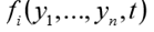 for a given independent argument t. In fact, the function func (y, t) implements the calculation of the right-hand sides of the system (1).
 The second argument y0 of the odeint () function is an array (or list) of initial values
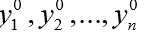 at t = t0.
 The third argument is an array of points in time at which you want a solution to the problem. In this case, the first element of this array is considered as t0.
The odeint () function returns an array of size len (t) x len (y0). The odeint () function has many options that control its operation. The rtol (relative error) and atol (absolute error) options determine the calculation error ei for each value of yi using the formula
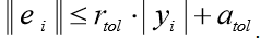
They can be vectors or scalars. Default

The ode ()
Function The second function of the scipy.integrate module, which is designed to solve differential equations and systems, is called ode (). It creates an ODU object (type scipy.integrate._ode.ode). Having reference to such an object, its methods should be used to solve differential equations. Similar to the odeint () function, the ode (func) function assumes the reduction of a problem to a system of differential equations of the form (1) and the use of its right-hand side function.
The only difference is that the function of the right-hand sides func (t, y) takes the independent variable as the first argument, and the second as the list of values of the desired functions. For example, the following sequence of instructions creates an ODE object representing the Cauchy task.
The Runge – Kutta method
When constructing numerical algorithms, we assume that the solution to this differential problem exists, it is unique and has the necessary smoothness properties.
In the numerical solution of the Cauchy problem
 (2)
(2)  (3)
(3) using the well-known solution at the point t = 0, it is necessary to find a solution for other t from equation (3). In the numerical solution of problem (2), (3), we will use a uniform, for simplicity, grid with variable t with step m> 0.
Approximate solution of problem (2), (3) at the point
 denote
  . The method converges at the point
  if
if 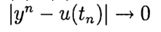 at
at  . The method has the pth order of accuracy if
 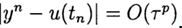 , p> 0 for . The simplest difference scheme for the approximate solution of problem (2), (3) is
  (4)
(4) If
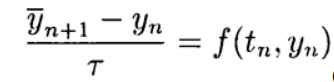
 we have an explicit method, in this case the difference scheme approximates equation (2) with first order. The symmetric scheme
  in (4) has the second order of approximation. This scheme belongs to the class of implicit ones — to determine an approximate solution on a new layer, it is necessary to solve a nonlinear problem.
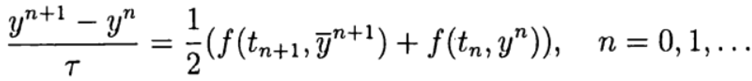
 Explicit schemes of the second and higher order approximations can be conveniently constructed based on the predictor-corrector method. At the stage of predictor (prediction), an explicit scheme is used
 (5)
(5)and at the corrector (refinement) stage, the scheme
In the one-step Runge — Kutt methods, the ideas of the predictor-corrector are implemented most fully. This method is written in the general form:
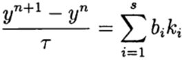 (6),
(6), where
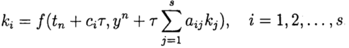
Formula (6) is based on s calculations of the function f and is called s-stage. If
 when
when  we have an explicit Runge-Kutta method. If for j> 1 and
  then it
  is determined implicitly from the equation:
 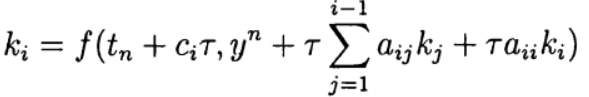 (7)
(7) This Runge – Kutta method is referred to as being diagonally implicit. Parameters
 define a variant of the Runge – Kutta method. The following method representation is used (the Butcher table).
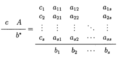
One of the most common is the explicit fourth-order Runge – Kutta method
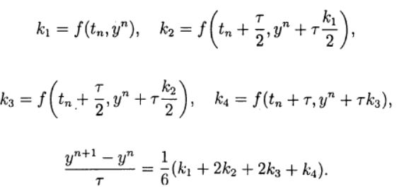 (8)
(8) The Runge – Kutta – Felberg method
I quote the value of the calculated coefficients of the
method  (9)
(9) Taking into account (9) the general solution is:
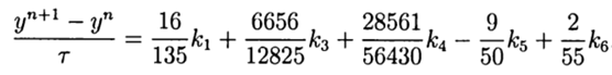 (10)
(10) This solution provides the fifth order of accuracy, it remains to adapt it to Python.
Computational experiment to determine the absolute error of the numerical solution of a nonlinear differential equation 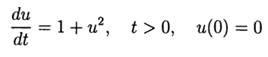 using both the def odein (), def oden () functions of the scipy.integrate module and the Runge – Kutta and Runge – Kutta methods adapted to Python
Program listing
from numpy import*
import matplotlib.pyplot as plt
from scipy.integrate import *
defodein():#dy1/dt=y2#dy2/dt=y1**2+1:deff(y,t):return y**2+1
         t =arange(0,1,0.01)
         y0 =0.0
         y=odeint(f, y0,t)
         y = array(y).flatten()
         return y,t
defoden():
         f = lambda t, y: y**2+1
         ODE=ode(f)
         ODE.set_integrator('dopri5')
         ODE.set_initial_value(0, 0)
         t=arange(0,1,0.01)
         z=[]
         t=arange(0,1,0.01)
         for i in arange(0,1,0.01):
                  ODE.integrate(i)
                  q=ODE.y
                  z.append(q[0])
         return z,t
defrungeKutta(f, to, yo, tEnd, tau):defincrement(f, t, y, tau):if z==1:
                           k0 =tau* f(t,y)
                           k1 =tau* f(t+tau/2.,y+k0/2.)
                           k2 =tau* f(t+tau/2.,y+k1/2.)
                           k3 =tau* f(t+tau, y + k2)
                           return (k0 + 2.*k1 + 2.*k2 + k3) / 6.elif z==0:
                           k1=tau*f(t,y)
                           k2=tau*f(t+(1/4)*tau,y+(1/4)*k1)
                           k3 =tau *f(t+(3/8)*tau,y+(3/32)*k1+(9/32)*k2)
                           k4=tau*f(t+(12/13)*tau,y+(1932/2197)*k1-(7200/2197)*k2+(7296/2197)*k3)
                           k5=tau*f(t+tau,y+(439/216)*k1-8*k2+(3680/513)*k3 -(845/4104)*k4)
                           k6=tau*f(t+(1/2)*tau,y-(8/27)*k1+2*k2-(3544/2565)*k3 +(1859/4104)*k4-(11/40)*k5)
                           return (16/135)*k1+(6656/12825)*k3+(28561/56430)*k4-(9/50)*k5+(2/55)*k6
         t = []
         y= []
         t.append(to)
         y.append(yo)
         while to < tEnd:
                  tau = min(tau, tEnd - to)
                  yo = yo + increment(f, to, yo, tau)
                  to = to + tau
                  t.append(to)
                  y.append(yo)
         return array(t), array(y)
deff(t, y):
         f = zeros([1])
         f[0] = y[0]**2+1return f
to = 0.
tEnd = 1
yo = array([0.])
tau = 0.01
z=1
t, yn = rungeKutta(f, to, yo, tEnd, tau)
y1n=[i[0] for i in yn]
plt.figure()
plt.title("Абсолютная погрешность численного решения(т.р.- u(t)=tan(t)) ДУ\n\
du/dt=u**2+1 c u(0)=0 при t>0")
plt.plot(t,abs(array(y1n)-array(tan(t))),label='Метод Рунге—Кутта \n\
четвертого порядка - расчёт по алгоритму')
plt.xlabel('Время')
plt.ylabel('Абсолютная погрешность.')
plt.legend(loc='best')
plt.grid(True)
z=0
t, ym = rungeKutta(f, to, yo, tEnd, tau)
y1m=[i[0] for i in ym]
plt.figure()
plt.title("Абсолютная погрешность численного решения(т.р.- u(t)=tan(t)) ДУ\n\
du/dt=u**2+1 c u(0)=0 при t>0")
plt.plot(t,abs(array(y1m)-array(tan(t))),label='Метод Рунге—Кутта— Фельберга \n\
пятого порядка - расчёт по алгоритму')
plt.xlabel('Время')
plt.ylabel('Абсолютная погрешность.')
plt.legend(loc='best')
plt.grid(True)
plt.figure()
plt.title("Абсолютная погрешность численного решения (т.р.- u(t)=tan(t)) ДУ\n\
du/dt=u**2+1 c u(0)=0 при t>0")
y,t=odein()
plt.plot(t,abs(array(tan(t))-array(y)),label='Функция odein')
plt.xlabel('Время')
plt.ylabel('Абсолютная погрешность.')
plt.legend(loc='best')
plt.grid(True)
plt.figure()
plt.title("Абсолютная погрешность численного решения (т.р.- u(t)=tan(t)) ДУ\n\
du/dt=u**2+1 c u(0)=0 при t>0")
z,t=oden()
plt.plot(t,abs(tan(t)-z),label='Функция ode метод Рунге—Кутта— Фельберга \n\
пятого порядка')
plt.xlabel('Время')
plt.ylabel('Абсолютная погрешность.')
plt.legend(loc='best')
plt.grid(True)
plt.show()
We get:
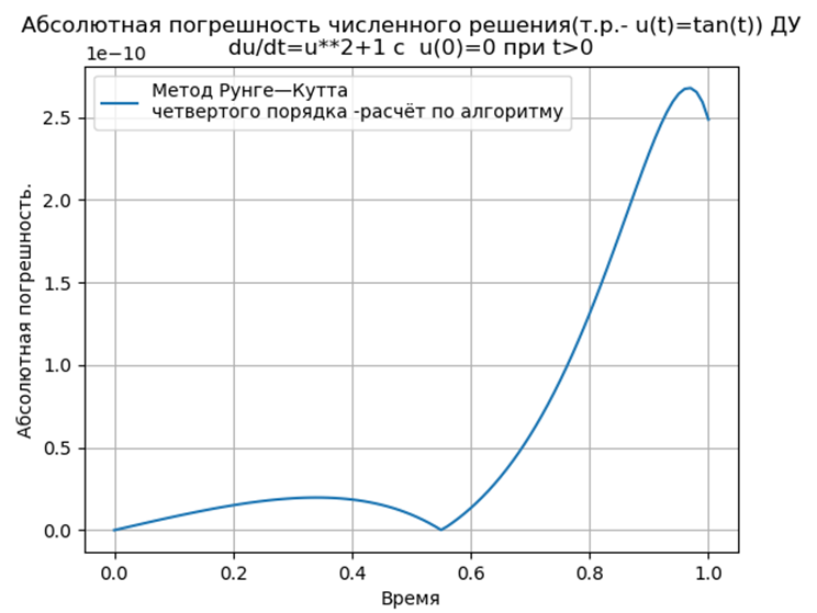
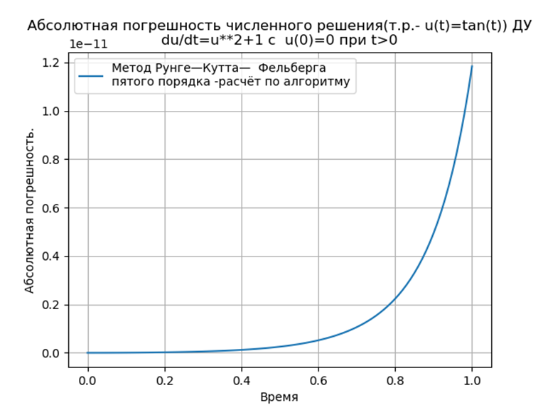
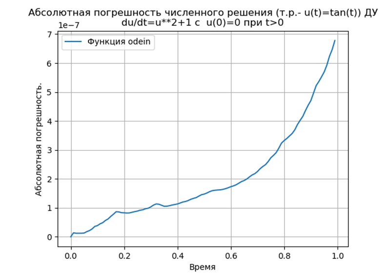
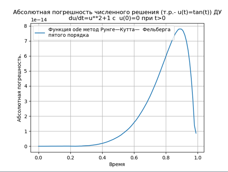
Conclusion: The
Runge – Kutta and Runge – Kutta – Felberg methods adapted to Python have a smaller absolute solution than using the odeint function, but more than using the edu function. It is necessary to conduct a performance study.
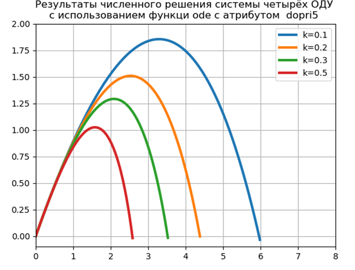
Численный эксперимент по сравнению быстродействия численного решения СДУ при использовании функции ode с атрибутом dopri5 (метод Рунге – Кутты 5 порядка) и с использованием адаптированного к Python метода Рунге—Кутта— Фельберга
Comparative analysis will be conducted on the example of the model problem given in [2]. In order not to repeat the source, I will give the formulation and solution of the model problem from [2].
We solve the Cauchy problem, which describes the motion of a body thrown with an initial velocity v0 at an angle α to the horizon under the assumption that air resistance is proportional to the square of the velocity. In the vector form, the equation of motion has the form
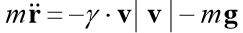
where
 is the radius of the vector of the moving body,
  is the velocity vector of the body,
  is the drag coefficient, the
  force vector of the weight of the body of mass m, g is the acceleration of gravity.
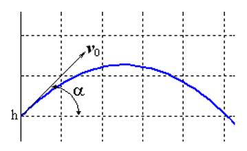
The peculiarity of this task is that the movement ends at an unknown moment of time when the body falls to the ground. If to designate
 , The coordinate form we have a system of equations
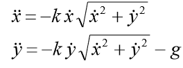
to the system should be added to the initial conditions:
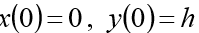 (h initial height)
  . Put
. Put 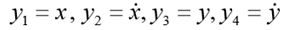 . Then the corresponding first-order ODE system takes the form: We set
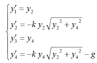
for the model problem
 . Omitting a rather extensive description of the program, I will give only a listing from the comments to which, I think, the principle of its operation will be clear. The program added countdown time for comparative analysis.
Program listing
import numpy as np
import matplotlib.pyplot as plt
import time
start = time.time()
from scipy.integrate import ode
ts = [ ]
ys = [ ]
FlightTime, Distance, Height =0,0,0
y4old=0deffout(t, y):# обработчик шага global FlightTime, Distance, Height,y4old
         ts.append(t)
         ys.append(list(y.copy()))
         y1, y2, y3, y4 = y
         if y4*y4old<=0:  # достигнута точка максимума
                  Height=y3
         if y4<0and y3<=0.0: # тело достигло поверхности
                  FlightTime=t
                  Distance=y1
                  return-1
         y4old=y4
# функция правых частей системы ОДУdeff(t, y, k):#  имеется дополнительный аргумент k
         g=9.81
         y1, y2, y3, y4 = y
         return [y2,-k*y2*np.sqrt(y2**2+y4**2), y4,-k*y4*np.sqrt(y2**2+y4**2)-g]
tmax=1.41# максимально допустимый момент времени
alph=np.pi/4# угол бросания тела
v0=10.0# начальная скорость
K=[0.1,0.2,0.3,0.5] # анализируемые коэффициенты сопротивления
y0,t0=[0, v0*np.cos(alph), 0, v0*np.sin(alph)], 0# начальные условия
ODE=ode(f)
ODE.set_integrator('dopri5', max_step=0.01)
ODE.set_solout(fout)
fig, ax = plt.subplots()
fig.set_facecolor('white')
for k in K:   # перебор значений коэффициента сопротивления
         ts, ys = [ ],[ ]
         ODE.set_initial_value(y0, t0) # задание начальных значений
         ODE.set_f_params(k)  # передача дополнительного аргумента k     # в функцию f(t,y,k) правых частей системы ОДУ
         ODE.integrate(tmax)      # решение ОДУ
         print('Flight time = %.4f Distance = %.4f Height =%.4f '% (FlightTime,Distance,Height))
         Y=np.array(ys)
         plt.plot(Y[:,0],Y[:,2],linewidth=3,label='k=%.1f'% k)
stop = time.time()
plt.title("Результаты численного решения системы четырёх ОДУ \n с использованием функци ode с атрибутом  dopri5  ")
print ("Время на модельную задачу: %f"%(stop-start))
plt.grid(True)
plt.xlim(0,8)
plt.ylim(-0.1,2)
plt.legend(loc='best')
plt.show()
We
get : Flight time = 1.2316 Distance = 5.9829 Height = 1.8542
Flight time = 1.1016 Distance = 4.3830 Height = 1.5088
Flight time = 1.0197 Distance = 3.5265 Height = 1.2912
Flight time = 0.9068 Distance = 2.5842 Height = 1.0240
Time for a model task: 0.454787
To implement Python tools for the numerical solution of the CDS without the use of special modules, I have proposed and investigated the following function: The increment function (f, t, y, tau) provides the fifth order of the numerical solution method. The remaining features of the program can be found in the following listing:
def increment(f, t, y, tau

 k1=tau*f(t,y)

 k2=tau*f(t+(1/4)*tau,y+(1/4)*k1)

 k3 =tau *f(t+(3/8)*tau,y+(3/32)*k1+(9/32)*k2)

 k4=tau*f(t+(12/13)*tau,y+(1932/2197)*k1-(7200/2197)*k2+(7296/2197)*k3)

 k5=tau*f(t+tau,y+(439/216)*k1-8*k2+(3680/513)*k3 -(845/4104)*k4)

 k6=tau*f(t+(1/2)*tau,y-(8/27)*k1+2*k2-(3544/2565)*k3 +(1859/4104)*k4-(11/40)*k5)

 return (16/135)*k1+(6656/12825)*k3+(28561/56430)*k4-(9/50)*k5+(2/55)*k6
Program listing
from numpy import*
import matplotlib.pyplot as plt
import time
start = time.time()
defrungeKutta(f, to, yo, tEnd, tau):defincrement(f, t, y, tau):# поиск приближённого решения методом Рунге—Кутта—Фельберга.
                  k1=tau*f(t,y)
                  k2=tau*f(t+(1/4)*tau,y+(1/4)*k1)
                  k3 =tau *f(t+(3/8)*tau,y+(3/32)*k1+(9/32)*k2)
                  k4=tau*f(t+(12/13)*tau,y+(1932/2197)*k1-(7200/2197)*k2+(7296/2197)*k3)
                  k5=tau*f(t+tau,y+(439/216)*k1-8*k2+(3680/513)*k3 -(845/4104)*k4)
                  k6=tau*f(t+(1/2)*tau,y-(8/27)*k1+2*k2-(3544/2565)*k3 +(1859/4104)*k4-(11/40)*k5)
                  return (16/135)*k1+(6656/12825)*k3+(28561/56430)*k4-(9/50)*k5+(2/55)*k6
         t = []#подготовка пустого списка t
         y= []#подготовка пустого списка y
         t.append(to)#внесение в список t начального значения to
         y.append(yo)#внесение в список y начального значения yowhile to < tEnd:#внесение результатов расчёта в массивы t,y
                  tau = min(tau, tEnd - to)#определение минимального шага tau
                  yo = yo + increment(f, to, yo, tau) # расчёт значения в точке t0,y0 для задачи Коши
                  to = to + tau # приращение времени
                  t.append(to) # заполнение массива t
                  y.append(yo) # заполнение массива y       return array(t), array(y)
deff(t, y):# функция правых частей системы ОДУ
         f = zeros([4])
         f[0]=y[1]
         f[1]=-k*y[1]*sqrt(y[1]**2+y[3]**2)
         f[2]=y[3]
         f[3]=-k*y[3]*sqrt(y[1]**2+y[3]**2) -g
         if y[3]<0and y[2]<=0.0: # тело достигло поверхностиreturn-1return f
to = 0# начальный момент отсчёта времени
tEnd = 1.41# конечный момент отсчёта времени
alph=pi/4# угол бросания тела
v0=10.0# начальная скорость
K=[0.1,0.2,0.3,0.5]# анализируемые коэффициенты сопротивления среды
g=9.81
yo = array([0.,v0*cos(alph),0.,v0*sin(alph)]) # начальные условия
tau =0.01# шагfor i in K:  # перебор значений коэффициента сопротивления среды
         k=i
         t, y = rungeKutta(f, to, yo, tEnd, tau)
         y1=array([i[0] for i in y]) # извлечение переменных из массива y
         y3=array([i[2] for i in y])
         # визуализация сопротивление среды "к" и расчёт и визуализация s,h,t
         plt.plot(y1,y3,linewidth=2,label='k=%.1f  h=%.3f  s=%.2f  t=%s' % (k,max(y3),max(y1),round(t[list(y1).index(max(y1))],3)))
stop = time.time()
plt.title("Результаты численного решения системы четырёх ОДУ \n с использованием адаптированного для Python\n метода Рунге—Кутта—Фельберга ")
print ("Время на модельную задачу: %f"%(stop-start))
plt.xlabel('Высота h')
plt.ylabel('Расстояние s')
plt.legend(loc='best')
plt.xlim(0,8)
plt.ylim(-0.1,2)
plt.grid(True)
plt.show()
We
get : Time for a model problem: 0.259927
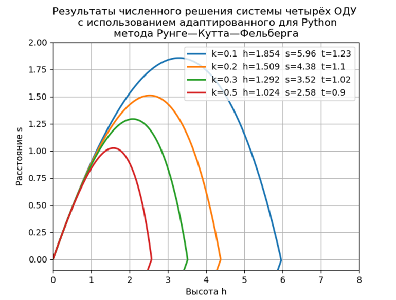
Conclusion The
proposed software implementation of a model problem without using special modules is almost twice as fast as with the ode function, but we must not forget that ode has a higher accuracy of the numerical solution and the possibility of choosing a solution method.
Solution of a boundary value problem with continuously separated boundary conditions
Let us give an example of some concrete boundary value problem with streamlined separated boundary conditions:
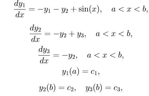 (11)
(11) To solve problem (11), we use the following algorithm:
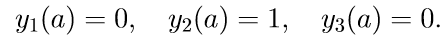
1. We solve the first three inhomogeneous equations of system (11) with initial conditions.

We introduce the notation to solve the Cauchy problem:
2. We solve the first three homogeneous system (11) with the initial conditions
introduce the notation for the solution of the Cauchy problem:
3. solve the first three homogeneous equations of the system (11) with the initial conditions

introduce the notation for the solution of the Cauchy problem:

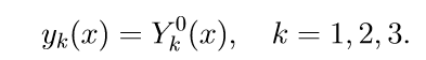
4. The general solution of the boundary value problem (11) using a solution of the Cauchy problem is written as a linear combination of solutions:

where p2, p3 - some unknown parameters.
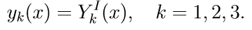
5. To determine the parameters p2 and p3, we use the boundary conditions of the last two equations (11), that is, the conditions for x = b. Substituting, we obtain a system of linear equations for the unknowns p2, p3:
 (12)
(12) Solving (12), we obtain the relations for p2, p3.
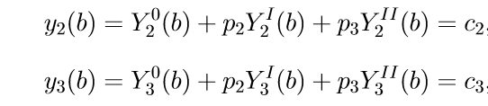
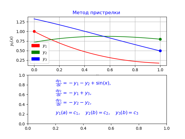
Using the above algorithm, using the Runge – Kutt – Felberg method, we obtain the following program:
Program listing
# Метод пристрелкиfrom numpy  import*
import matplotlib.pyplot as plt
import matplotlib.font_manager as fm,os
import matplotlib.patches as mpatches
import matplotlib.lines as mlines
from scipy.integrate import odeint
from scipy import linalg
import time
start = time.time()
c1 = 1.0
c2 = 0.8
c3 = 0.5
a =0.0
b = 1.0
nn =100
initial_state_0 =array( [a, c1, 0.0, 0.0])
initial_state_I =array( [a, 0.0, 1.0, 0.0])
initial_state_II =array( [a, 0.0, 0.0, 1.0])
to = a
tEnd =b
N = int(nn)
tau=(b-a)/N
defrungeKutta(f, to, yo, tEnd, tau):defincrement(f, t, y, tau):
                  k1=tau*f(t,y)
                  k2=tau*f(t+(1/4)*tau,y+(1/4)*k1)
                  k3 =tau *f(t+(3/8)*tau,y+(3/32)*k1+(9/32)*k2)
                  k4=tau*f(t+(12/13)*tau,y+(1932/2197)*k1-(7200/2197)*k2+(7296/2197)*k3)
                  k5=tau*f(t+tau,y+(439/216)*k1-8*k2+(3680/513)*k3 -(845/4104)*k4)
                  k6=tau*f(t+(1/2)*tau,y-(8/27)*k1+2*k2-(3544/2565)*k3 +(1859/4104)*k4-(11/40)*k5)
                  return (16/135)*k1+(6656/12825)*k3+(28561/56430)*k4-(9/50)*k5+(2/55)*k6
         t = []
         y= []
         t.append(to)
         y.append(yo)
         while to < tEnd:
                  tau = min(tau, tEnd - to)
                  yo = yo + increment(f, to, yo, tau)
                  to = to + tau
                  t.append(to)
                  y.append(yo)
         return array(t), array(y)
deff(t, y):global theta
         f = zeros([4])
         f[0] = 1
         f[1] = -y [1]-y[2] +theta* sin(y[0])
         f[2] = -y[2]+y[3]
         f[3] = -y[2]
         return f
# Решение НЕОДНОРОДНОЙ системы -- theta = 1
theta = 1.0
yo =initial_state_0
t, y = rungeKutta(f, to, yo, tEnd, tau)
y2=[i[2] for i in y]
y3=[i[3] for i in y]
# Извлечение требуемых для решения задачи значений # Y20 = Y2(b), Y30 = Y3(b)
Y20 = y2[N-1]
Y30 = y3[N-1]
# Решение ОДНОРОДНОЙ системы -- theta = 0, задача I
theta = 0.0
yo= initial_state_I
t, y = rungeKutta(f, to, yo, tEnd, tau)
y2=[i[2] for i in y]
y3=[i[3] for i in y]
# Извлечение требуемых для решения задачи значений # Y21= Y2(b), Y31 = Y3(b)
Y21= y2[N-1]
Y31 = y3[N-1]
# Решение ОДНОРОДНОЙ системы -- theta = 0, задача II
theta = 0.0
yo =initial_state_II
t, y = rungeKutta(f, to, yo, tEnd, tau)
y2=[i[2] for i in y]
y3=[i[3] for i in y]
# Извлечение требуемых для решения задачи значений # Y211= Y2(b), Y311 = Y3(b)
Y211= y2[N-1]
Y311 = y3[N-1]
# Формирование системы линейных# АЛГЕБРАИЧЕСКИХ уравнений для определния p2, p3
b1 = c2 - Y20
b2 = c3 - Y30
A = array([[Y21, Y211], [Y31, Y311]])
bb = array([[b1], [b2]])
 # Решение системы
p2, p3 = linalg.solve(A, bb)
# Окончательное решение краевой# НЕОДНОРОДНОЙ задачи, theta = 1
theta = 1.0
yo = array([a, c1, p2, p3])
t, y = rungeKutta(f, to, yo, tEnd, tau)
y0=[i[0] for i in y]
y1=[i[1] for i in y]
y2=[i[2] for i in y]
y3=[i[3] for i in y]
# Проверка
print('y0[0]=', y0[0])
print('y1[0]=', y1[0])
print('y2[0]=', y2[0])
print('y3[0]=', y3[0])
print('y0[N-1]=', y0[N-1])
print('y1[N-1]=', y1[N-1])
print('y2[N-1]=', y2[N-1])
print('y3[N-1]=', y3[N-1])
j = N
xx = y0[:j]
yy1 = y1[:j]
yy2 = y2[:j]
yy3 = y3[:j]
stop = time.time()
print ("Время на модельную задачу: %f"%(stop-start))
plt.subplot(2, 1, 1)
plt.plot([a], [c1], 'ro')
plt.plot([b], [c2], 'go')
plt.plot([b], [c3], 'bo')
plt.plot(xx, yy1, color='r') #Построение графика
plt.plot(xx, yy2, color='g') #Построение графика
plt.plot(xx, yy3, color='b') #Построение графика
plt.xlabel(r'$x$') #Метка по оси x в формате TeX
plt.ylabel(r'$y_k(x)$') #Метка по оси y в формате TeX
plt.title(r'Метод пристрелки ', color='blue')
plt.grid(True) #Сетка
patch_y1 = mpatches.Patch(color='red',
                          label='$y_1$')
patch_y2 = mpatches.Patch(color='green',
                          label='$y_2$')
patch_y3 = mpatches.Patch(color='blue',
                           label='$y_3$')
plt.legend(handles=[patch_y1, patch_y2, patch_y3])
ymin, ymax = plt.ylim()
xmin, xmax = plt.xlim()
plt.subplot(2, 1, 2)
font = {'family': 'serif',
        'color': 'blue',
        'weight': 'normal',
        'size': 12,
        }
plt.text(0.2, 0.8, r'$\frac{dy_1}{dx}= - y_1 - y_2 + \sin(x),$',
         fontdict=font)
plt.text(0.2, 0.6,r'$\frac{dy_2}{dx}= - y_1 + y_3,$',
         fontdict=font)
plt.text(0.2, 0.4, r'$\frac{dy_3}{dx}= - y_2 - y_2,$',
         fontdict=font)
plt.text(0.2, 0.2, r'$y_1(a)=c_1, 'r'\quad y_2(b)=c_2, \quad y_3(b)=c_3.$',
         fontdict=font)
plt.subplots_adjust(left=0.15)
plt.show()
We get:
y0 [0] = 0.0
y1 [0] = 1.0
y2 [0] = 0.7156448588231397
y3 [0] = 1.324566562303714
y0 [N-1] = 0.9900000000000007
y1 [N-1] = 0.1747719838716767
y2 [N-1] = 0.8
y3 [N-1] = 0.5000000000000001
Time for a model problem: 0.070878
Conclusion
The program I developed differs from the smaller error given in [3], which confirms the comparative analysis of the odeint function given at the beginning of the article with the Runge – Kutt – Feelberg method implemented in Python.
References:
1. Numerical solution of mathematical models of objects defined by composite systems of differential equations.
2. Introduction to Scientific Python.
3. N.M. Polyakova, E.V. Shiryaeva Python 3. Creating a graphical user interface (by the example of solving the boundary-value problem for linear ordinary differential equations using the method of adjustment). Rostov-on-Don 2017.