Local rate of training of neuron weights in the backpropagation algorithm
Hi, in one of the last lectures on neural networks on the cursor, we talked about how to improve the convergence of the error back propagation algorithm in general, and in particular, we examined a model where each neuron weight has its own learning rate (neuron local gain). I have long wanted to implement some kind of algorithm that would automatically adjust the speed of network learning, but all laziness did not reach my hands, and then suddenly such a simple and uncomplicated method. In this short article I will talk about this model and give some examples of when this model can be useful.
Let's start with the theory, first we’ll recall what a change in one weight is equal to, in this case with regularization, but it doesn’t change the essence:

In the basic case, training speed is a global parameter for all weights.
We introduce a training speed modifier for each weight of each neuron , and we will change the weights of neurons according to the following rule:

At the first training session, all training speed modifiers are equal to one, then the dynamic tuning of the modifiers in the learning process is as follows:
It makes sense to make the bonus a very small number less than unity, and the penalty , thus b + p = 1. For example, a = 0.05, p = 0.95. This setting ensures that in the case of an oscillation of the direction of the gradient vector, the modifier value will tend back to the initial unit. If you do not go into mathematics, then we can say that the algorithm encourages those weights (growth within the framework of some dimension of the space of weights) that retain their direction relative to the previous point in time, and fines those who start to rush about.
The author of this method, Geoffrey Hinton (by the way, he was one of the first to use gradient descent to train a neural network) also advises taking into account the following things:
All experiments were carried out on a set of 29 by 29 pixel pictures on which English letters were drawn. One hidden layer of 100 neurons with a sigmoid activation function was used, the softmax layer was at the output , and cross entropy was minimized. In total, it is easy to calculate that there are 100 * (29 * 29 + 1) + 26 * (100 + 1) = 86826 weights in the network (including offsets). The initial values of the weights were taken from a uniform distribution . All three experiments used the same weight initialization. Full batch is also used.
In this experiment, a simple, easily generalizable set was used; the value of the learning speed (global speed) is 0.01 . Consider the dependence of the value of the network error on the data from the era of training.
It can be seen that on a very simple set there is a positive effect of the modifier, but it is not great.
In contrast to the first experiment, I took a lot, which I already somehow taught. I was aware in advance that with a learning speed of 0.01 , the oscillation of the value of the error function starts very quickly, and with a lower value, the set is generalized. But in this test it will be used exactly 0.01 , because I want to see what happens.
A complete failure! The modifier not only did not improve the quality, but on the contrary, it increased the oscillation, while without the modifier, the error decreases on average.
In this experiment, I use the same set as in the second, but the global learning speed is 0.001 .
In this case, we get a very significant increase in quality. And if, after 300 eras, drive out recognition on the training set and test:
And I made one conclusion for myself that this method is not a substitute for choosing the global learning speed, but is a good addition to the already selected training speed.
Theory
Let's start with the theory, first we’ll recall what a change in one weight is equal to, in this case with regularization, but it doesn’t change the essence:
- this (η) is the speed of learning
- m is the size of the training set
- n - layer number
- full notation here
In the basic case, training speed is a global parameter for all weights.
We introduce a training speed modifier for each weight of each neuron
, and we will change the weights of neurons according to the following rule: At the first training session, all training speed modifiers are equal to one, then the dynamic tuning of the modifiers in the learning process is as follows:
 - the value of the gradient at a certain point in time
- tau τ - current time point or current training batch
- b - the additive bonus that the modifier receives if the direction of the gradient for a certain dimension does not change
- p - multiplicative penalty, in the case of a change in the direction of the gradient vector
It makes sense to make the bonus a very small number less than unity, and the penalty
, thus b + p = 1. For example, a = 0.05, p = 0.95. This setting ensures that in the case of an oscillation of the direction of the gradient vector, the modifier value will tend back to the initial unit. If you do not go into mathematics, then we can say that the algorithm encourages those weights (growth within the framework of some dimension of the space of weights) that retain their direction relative to the previous point in time, and fines those who start to rush about. The author of this method, Geoffrey Hinton (by the way, he was one of the first to use gradient descent to train a neural network) also advises taking into account the following things:
- first, set reasonable growth limits for modifiers
- secondly, you should not use this technique for online training, or for small batches; it is necessary that during the batch process a fairly general gradient would accumulate; otherwise, the direction oscillation frequency increases, and thereby the meaning in the modifier is lost
The experiments
All experiments were carried out on a set of 29 by 29 pixel pictures on which English letters were drawn. One hidden layer of 100 neurons with a sigmoid activation function was used, the softmax layer was at the output , and cross entropy was minimized. In total, it is easy to calculate that there are 100 * (29 * 29 + 1) + 26 * (100 + 1) = 86826 weights in the network (including offsets). The initial values of the weights were taken from a uniform distribution
. All three experiments used the same weight initialization. Full batch is also used.First
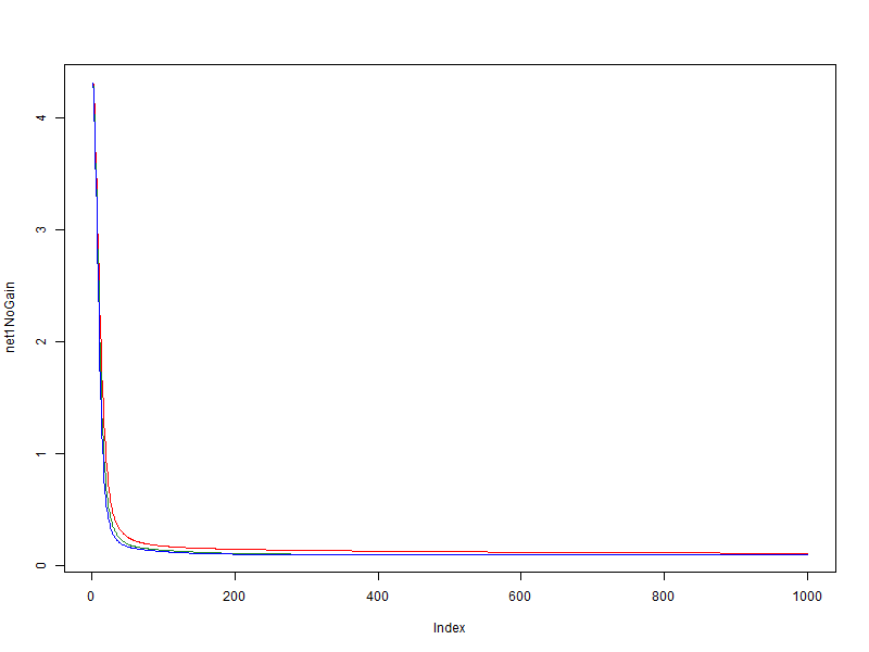
In this experiment, a simple, easily generalizable set was used; the value of the learning speed (global speed) is 0.01 . Consider the dependence of the value of the network error on the data from the era of training.
- red - without using a modifier
- green - bonus = 0.05, penalty = 0.95, limit = [0.1, 10]
- blue - bonus = 0.1, penalty = 0.9, limit = [0.01, 100]
It can be seen that on a very simple set there is a positive effect of the modifier, but it is not great.
Second
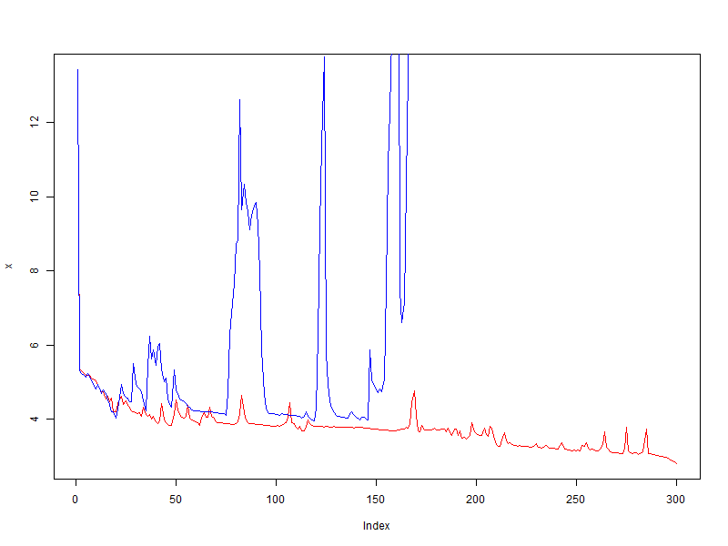
In contrast to the first experiment, I took a lot, which I already somehow taught. I was aware in advance that with a learning speed of 0.01 , the oscillation of the value of the error function starts very quickly, and with a lower value, the set is generalized. But in this test it will be used exactly 0.01 , because I want to see what happens.
- red - without using a modifier
- blue - bonus = 0.05, penalty = 0.95, limit = [0.1, 10]
A complete failure! The modifier not only did not improve the quality, but on the contrary, it increased the oscillation, while without the modifier, the error decreases on average.
Third
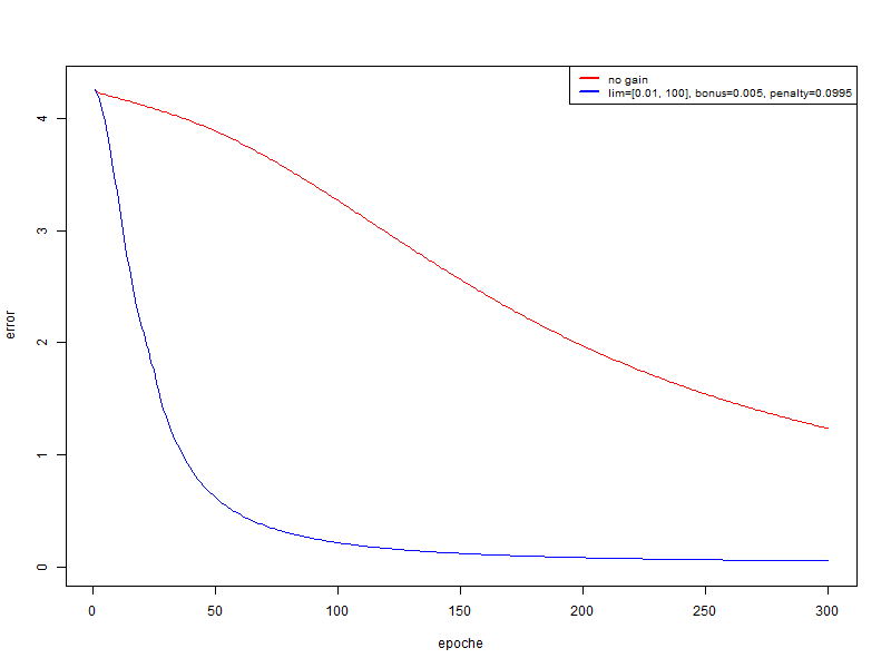
In this experiment, I use the same set as in the second, but the global learning speed is 0.001 .
- red - without using a modifier
- blue - bonus = 0.005, penalty = 0.995, limit = [0.01, 100]
In this case, we get a very significant increase in quality. And if, after 300 eras, drive out recognition on the training set and test:
- red: on the training set 94.74%, on the test 67.18%
- blue: on the training set 100%; on test 74.4%
Conclusion
And I made one conclusion for myself that this method is not a substitute for choosing the global learning speed, but is a good addition to the already selected training speed.