Optimizing the rendering of scenes from the Disney cartoon "Moana". Part 1
- Transfer
Walt Disney Animation Studios (WDAS) recently gave the rendering community an invaluable gift to the community by releasing a full scene description for the island from the Moana cartoon . Geometry and textures for a single frame occupy more than 70 GB of disk space. This is a terrific example of the degree of complexity that rendering systems have to deal with today; never before have researchers and developers engaged in rendering outside film studios been able to work with such realistic scenes.
Here is the result of rendering the scene using modern pbrt:
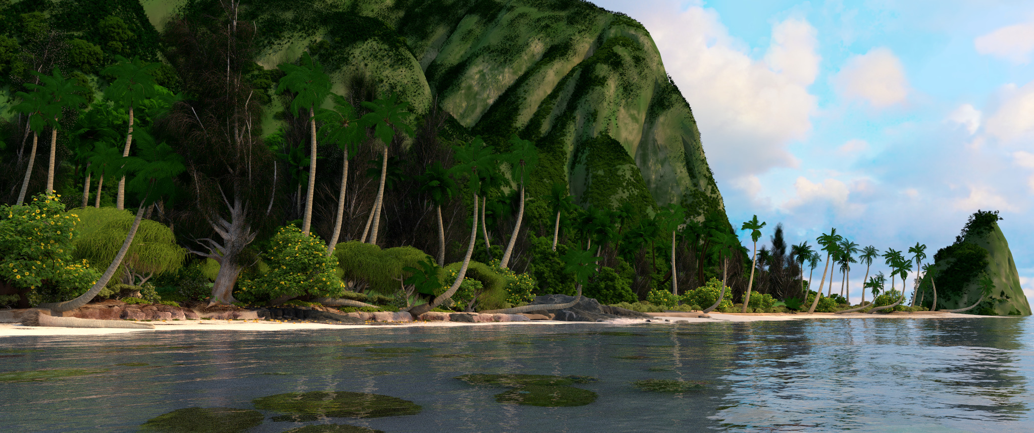
The island of "Moana", rendered pbrt-v3 in the resolution of 2048x858 with 256 samples per pixel. The total rendering time on a 12-core / 24-threaded Google Compute Engine instance with a frequency of 2 GHz with the latest version of pbrt-v3 was 1 h 44 min 45 s.
On the Disney side, it was a lot of work; it had to extract the scene from its own internal format and transform it into a regular one; Special thanks to her for the time spent on packaging and preparing this data for widespread use. I am confident that their work will be well rewarded in the future, because researchers use this scene to study the problems of effectively rendering scenes of this level of complexity.
This scene has already taught me a lot and allowed me to improve the pbrt renderer, but before we get to this, I’ll tell a short story to understand the context.
Many years ago, while going through an internship in the Pixar rendering team, I learned a curious lesson: “interesting” things almost always appear when input data are transferred to the software system that is significantly different from what it was before. Even in well-written and mature software systems, new types of input almost always lead to the detection of unknown defects in an existing implementation.
I first learned this lesson during the production of Toy Story 2 . One day, someone noticed that a surprisingly long amount of time was spent on parsing RIB scene description files. Someone else from the rendering team (I guess it was Craig Kolb) started the profiler and started to figure it out.
It turned out that most of the parsing time was taken up by searching the hash table used forstring interning . The hash table had a rather small size, probably 256 elements, and when several values were hashed into one cell, it organized the chain. After the first implementation of the hash table, a lot of time passed and now there were tens of thousands of objects in the scenes, so such a small table quickly filled up and became ineffective.
The most expedient way was to simply increase the size of the table - all this happened at the height of the workflow, so there was no time for any sophisticated solution, for example, expanding the size of the table when filling it. We make a change in one line, reassemble the application, perform a quick test before the commit and ... no speed improvements occur. The search for the hash table takes the same amount of time. Awesome!
After further study, it was found that the hash table function used was analogous to the following:
(Forgive me, Pixar, if I revealed your top-secret source code RenderMan.)
The hash function was implemented back in the 1980s. At that time, the programmer probably thought that the computational cost of checking the effect of all characters on the string on the hash value would be too high and not worth it. (I think that if there were only a few objects in the scene and 256 elements in the hash table, then this was quite enough.)
Another obsolete implementation also contributed: since the moment Pixar started creating its films, the names of objects in the scenes have grown quite a bit, for example, “BuzzLightyear / LeftArm / Hand / IndexFinger / Knuckle2”. However, some initial stage of the pipeline used to store the names of objects a fixed-length buffer and shortened all long names, retaining only the end, and, if lucky, added an ellipsis at the beginning, making it clear that part of the name was lost: "... year / LeftArm / Hand / IndexFinger / Knuckle2 ".
Subsequently, all the names of objects that the renderer saw had this form, the hash function hashed them all into one memory fragment as ".", And the hash table was actually a large linked list. Good old days. At least, having understood, we rather quickly corrected this error.
I remembered this lesson last year, when Heather Pritchet and Rasmus Tamstorf from WDAS contacted me and asked if I would be interested to check the possible rendering quality of the scene from Moana in pbrt 1 . Naturally, I agreed. I was glad to help and I was wondering how everything will turn out.
The naive optimist inside me hoped that there would be no huge surprises - after all, the first version of pbrt was released about 15 years ago, and many people used and studied its code for many years. You can be sure that there will be no interference like the old hash function from RenderMan, right?
Of course, the answer was no. (And that is why I am writing this and several other posts.) Although I was a little disappointed that pbrt was not perfect out of the box, but I think that my experience with the scene from Moana was the first confirmation of the value of publishing this scene ; pbrt has already become a better system due to the fact that I figured out the processing of this scene.
Having access to the scene, I immediately downloaded it (with my home Internet connection, it took several hours) and unpacked from tar, receiving 29 GB of pbrt files and 38 GB of ptex 2 texture maps . I blithely tried to render the scene on my home system (with 16 GB of RAM and a 4-core CPU). Returning after a while to the computer, I saw that it hung, all the RAM is full, and pbrt is still trying to complete the parsing of the scene description. The OS was trying to cope with the task using virtual memory, but it seemed hopeless. Having nailed the process, I had to wait about a minute before the system began to respond to my actions.
The next attempt was the Google Compute Engine instance, which allows you to use more RAM (120 GB) and more CPUs (32 threads per 16 CPUs). The good news was that pbrt was able to successfully render the scene (thanks to the work of Heather and Rasmus in translating it into pbrt format). It was very exciting to see that pbrt can generate relatively good pixels for high-quality movie content, but the speed was not so exciting: 34 min 58 s only for parsing the scene description, and the system spent up to 70 GB of RAM during rendering.
Yes, the disk contained 29 gigabytes of pbrt scene description files that needed to be parsed, so I did not expect the first stage to take a couple of seconds. But spend half an hour before the rays begin to be traced? This greatly complicates the work with the scene.
On the other hand, such speed told us that something very badly smelling was probably happening in the code; not just “matrix inversion can be done 10% faster”; rather, something of the level of "oh, we go through a linked list of 100 thousand items." I was optimistic and hoped that by understanding, I could speed up the process considerably.
The first place I started looking for clues was the pbrt dump statistics after rendering. The main stages of the execution of pbrt are configured so that you can collect approximate data profiling by fixing operations with periodic interruptions in the rendering process. Unfortunately, the statistics did not help us much: according to reports, from almost 35 minutes before the start of rendering, 4 minutes and 22 seconds was spent on building BVH, but there was no detail about the rest of the time.
Building a BVH is the only significant computational task that is performed while the scene is parsing; all the rest is essentially a de-serialization of descriptions of geometry and materials. Knowing how much time was spent on creating BVH gave an understanding of how (not) the system was effective: the remaining time, namely about 30 minutes, spent on parsing 29 GB of data, that is, the speed was 16.5 MB / s. Well-optimized JSON parsers, in fact performing the same task, work at a speed of 50-200 MB / s. It is clear that there is still room for improvement.
To better understand what wasted time, I launched pbrt with the Linux perf tool.which never used before. But it seems that he coped with the task. I instructed him to look for the DWARF characters to get the function names (
Here is what he could tell me after starting with pbrt:
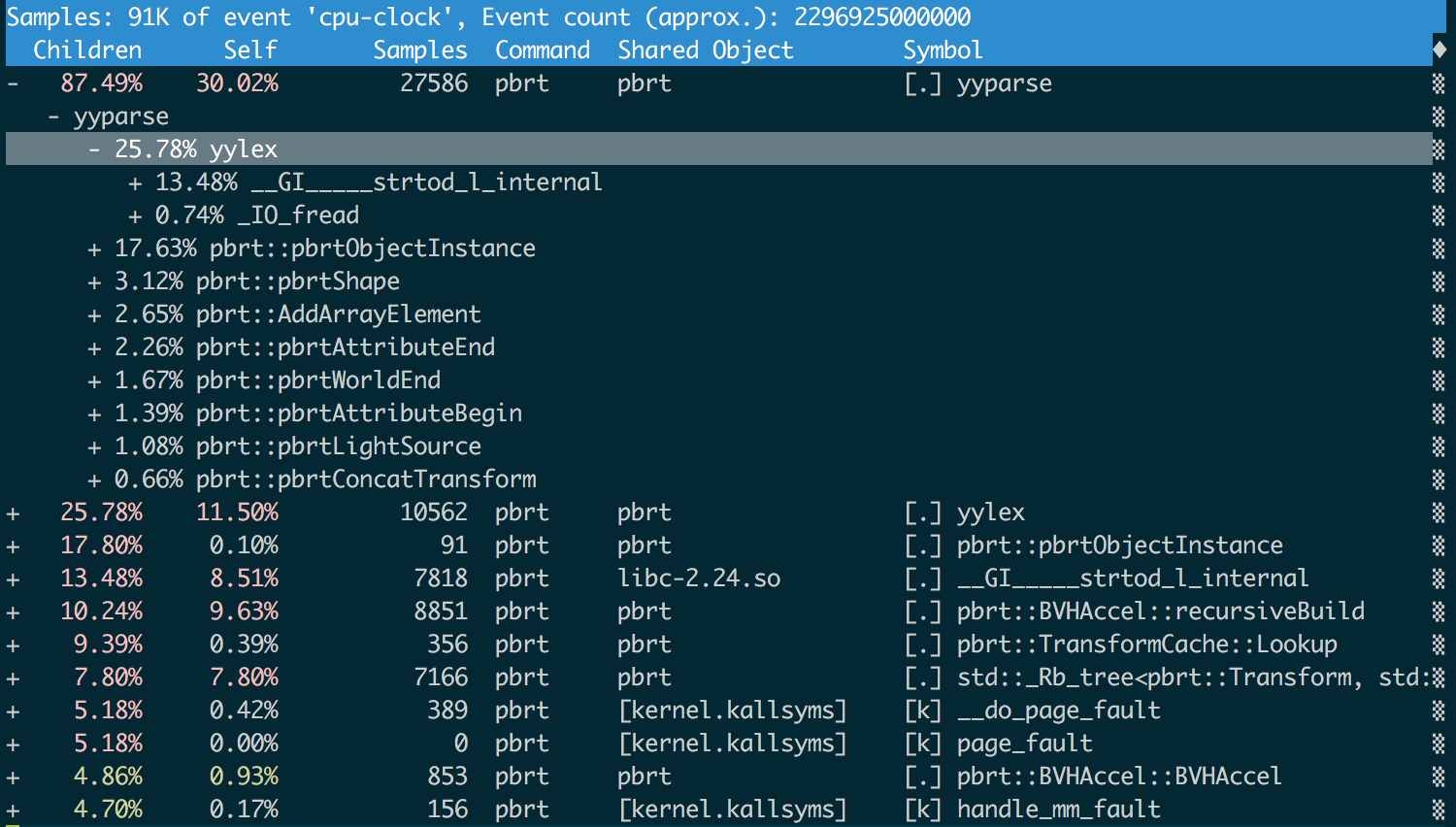
I was not joking when I talked about the “interface with nice curses”.
We see that more than half of the time is spent on the mechanics of parsing:
One way to spend less time parsing data in text form is to convert the data to a format that is parsed more efficiently. Quite a large part of the 29 GB of these scene description files are triangle meshes, and pbrt already has native support for the PLY format , which is an effective binary representation of polygonal meshes. Also in pbrt there is a command line flag
The catch is that ptex textures are used extensively in the Disney scene , which, in turn, require that each triangle have a value associated with it.
I wrote a small command line script to convert all files.
After converting all large meshes to PLY, the size of the scene description on the disk decreased from 29 to 22 GB: 16.9 GB of pbrt scene files and 5.1 GB of PLY binary files. After the conversion, the total time of the first stage of the system decreased to 27 minutes 35 seconds, and the savings amounted to 7 minutes 23 seconds, that is, we accelerated 1.3 times 3 . Processing a PLY file is much more efficient than processing a pbrt text file: just 40 seconds of the launch time was spent on parsing the PLY files, and we see that the PLY files were processed at a speed of about 130 MB / s, or about 8 times faster than the text format pbrt .
It was a good easy win, but we still had a lot to do.
The next time we'll figure out where all the memory is actually used, fix some bugs here, and achieve even more speed in the process.
Here is the result of rendering the scene using modern pbrt:
The island of "Moana", rendered pbrt-v3 in the resolution of 2048x858 with 256 samples per pixel. The total rendering time on a 12-core / 24-threaded Google Compute Engine instance with a frequency of 2 GHz with the latest version of pbrt-v3 was 1 h 44 min 45 s.
On the Disney side, it was a lot of work; it had to extract the scene from its own internal format and transform it into a regular one; Special thanks to her for the time spent on packaging and preparing this data for widespread use. I am confident that their work will be well rewarded in the future, because researchers use this scene to study the problems of effectively rendering scenes of this level of complexity.
This scene has already taught me a lot and allowed me to improve the pbrt renderer, but before we get to this, I’ll tell a short story to understand the context.
Hash which was not
Many years ago, while going through an internship in the Pixar rendering team, I learned a curious lesson: “interesting” things almost always appear when input data are transferred to the software system that is significantly different from what it was before. Even in well-written and mature software systems, new types of input almost always lead to the detection of unknown defects in an existing implementation.
I first learned this lesson during the production of Toy Story 2 . One day, someone noticed that a surprisingly long amount of time was spent on parsing RIB scene description files. Someone else from the rendering team (I guess it was Craig Kolb) started the profiler and started to figure it out.
It turned out that most of the parsing time was taken up by searching the hash table used forstring interning . The hash table had a rather small size, probably 256 elements, and when several values were hashed into one cell, it organized the chain. After the first implementation of the hash table, a lot of time passed and now there were tens of thousands of objects in the scenes, so such a small table quickly filled up and became ineffective.
The most expedient way was to simply increase the size of the table - all this happened at the height of the workflow, so there was no time for any sophisticated solution, for example, expanding the size of the table when filling it. We make a change in one line, reassemble the application, perform a quick test before the commit and ... no speed improvements occur. The search for the hash table takes the same amount of time. Awesome!
After further study, it was found that the hash table function used was analogous to the following:
inthash(constchar *str){
    return str[0];
}
(Forgive me, Pixar, if I revealed your top-secret source code RenderMan.)
The hash function was implemented back in the 1980s. At that time, the programmer probably thought that the computational cost of checking the effect of all characters on the string on the hash value would be too high and not worth it. (I think that if there were only a few objects in the scene and 256 elements in the hash table, then this was quite enough.)
Another obsolete implementation also contributed: since the moment Pixar started creating its films, the names of objects in the scenes have grown quite a bit, for example, “BuzzLightyear / LeftArm / Hand / IndexFinger / Knuckle2”. However, some initial stage of the pipeline used to store the names of objects a fixed-length buffer and shortened all long names, retaining only the end, and, if lucky, added an ellipsis at the beginning, making it clear that part of the name was lost: "... year / LeftArm / Hand / IndexFinger / Knuckle2 ".
Subsequently, all the names of objects that the renderer saw had this form, the hash function hashed them all into one memory fragment as ".", And the hash table was actually a large linked list. Good old days. At least, having understood, we rather quickly corrected this error.
Intriguing innovation
I remembered this lesson last year, when Heather Pritchet and Rasmus Tamstorf from WDAS contacted me and asked if I would be interested to check the possible rendering quality of the scene from Moana in pbrt 1 . Naturally, I agreed. I was glad to help and I was wondering how everything will turn out.
The naive optimist inside me hoped that there would be no huge surprises - after all, the first version of pbrt was released about 15 years ago, and many people used and studied its code for many years. You can be sure that there will be no interference like the old hash function from RenderMan, right?
Of course, the answer was no. (And that is why I am writing this and several other posts.) Although I was a little disappointed that pbrt was not perfect out of the box, but I think that my experience with the scene from Moana was the first confirmation of the value of publishing this scene ; pbrt has already become a better system due to the fact that I figured out the processing of this scene.
First renders
Having access to the scene, I immediately downloaded it (with my home Internet connection, it took several hours) and unpacked from tar, receiving 29 GB of pbrt files and 38 GB of ptex 2 texture maps . I blithely tried to render the scene on my home system (with 16 GB of RAM and a 4-core CPU). Returning after a while to the computer, I saw that it hung, all the RAM is full, and pbrt is still trying to complete the parsing of the scene description. The OS was trying to cope with the task using virtual memory, but it seemed hopeless. Having nailed the process, I had to wait about a minute before the system began to respond to my actions.
The next attempt was the Google Compute Engine instance, which allows you to use more RAM (120 GB) and more CPUs (32 threads per 16 CPUs). The good news was that pbrt was able to successfully render the scene (thanks to the work of Heather and Rasmus in translating it into pbrt format). It was very exciting to see that pbrt can generate relatively good pixels for high-quality movie content, but the speed was not so exciting: 34 min 58 s only for parsing the scene description, and the system spent up to 70 GB of RAM during rendering.
Yes, the disk contained 29 gigabytes of pbrt scene description files that needed to be parsed, so I did not expect the first stage to take a couple of seconds. But spend half an hour before the rays begin to be traced? This greatly complicates the work with the scene.
On the other hand, such speed told us that something very badly smelling was probably happening in the code; not just “matrix inversion can be done 10% faster”; rather, something of the level of "oh, we go through a linked list of 100 thousand items." I was optimistic and hoped that by understanding, I could speed up the process considerably.
Statistics don't help
The first place I started looking for clues was the pbrt dump statistics after rendering. The main stages of the execution of pbrt are configured so that you can collect approximate data profiling by fixing operations with periodic interruptions in the rendering process. Unfortunately, the statistics did not help us much: according to reports, from almost 35 minutes before the start of rendering, 4 minutes and 22 seconds was spent on building BVH, but there was no detail about the rest of the time.
Building a BVH is the only significant computational task that is performed while the scene is parsing; all the rest is essentially a de-serialization of descriptions of geometry and materials. Knowing how much time was spent on creating BVH gave an understanding of how (not) the system was effective: the remaining time, namely about 30 minutes, spent on parsing 29 GB of data, that is, the speed was 16.5 MB / s. Well-optimized JSON parsers, in fact performing the same task, work at a speed of 50-200 MB / s. It is clear that there is still room for improvement.
To better understand what wasted time, I launched pbrt with the Linux perf tool.which never used before. But it seems that he coped with the task. I instructed him to look for the DWARF characters to get the function names (
--call-graph dwarf), and in order not to get the staggering trace files, I had to reduce the sampling rate from 4,000 to 100 samples per second ( -F 100). But with these parameters, everything went great, and I was pleasantly surprised that the tool perf reporthas an interface with nice curses. Here is what he could tell me after starting with pbrt:
I was not joking when I talked about the “interface with nice curses”.
We see that more than half of the time is spent on the mechanics of parsing:
yyparse()is a parser generated by bison , and yylex()is a lexical analyzer (lexer) generated by flex . More than half the time is yylex()spent on strtod()converting strings to double values. We will postpone the attack on yyparse()and yylex()to the third article of this series, but now we can understand that reducing the amount of data thrown into the renderer can be a good idea.From text to PLY
One way to spend less time parsing data in text form is to convert the data to a format that is parsed more efficiently. Quite a large part of the 29 GB of these scene description files are triangle meshes, and pbrt already has native support for the PLY format , which is an effective binary representation of polygonal meshes. Also in pbrt there is a command line flag
--toplythat parses the scene description file pbrt, converts all the triangle meshes found into PLY files and creates a new pbrt file that references these PLY files. The catch is that ptex textures are used extensively in the Disney scene , which, in turn, require that each triangle have a value associated with it.
faceIndexthat determines from which face of the original subdivided mesh it is taken. To transfer these values, it was enough just to add support for new fields in the PLY file . Further research revealed that if each mesh is converted — even if there are only ten triangles in it — into the PLY file, tens of thousands of small PLY files are created in the folder, and this creates its own performance problems; We managed to get rid of this problem by adding to the implementation the ability to leave small meshes unchanged . I wrote a small command line script to convert all files.
*_geometry.pbrtin the folder to use PLY for large meshes. Note that it has hard-coded assumptions about the paths that need to be changed in order for the script to work elsewhere.First speed boost
After converting all large meshes to PLY, the size of the scene description on the disk decreased from 29 to 22 GB: 16.9 GB of pbrt scene files and 5.1 GB of PLY binary files. After the conversion, the total time of the first stage of the system decreased to 27 minutes 35 seconds, and the savings amounted to 7 minutes 23 seconds, that is, we accelerated 1.3 times 3 . Processing a PLY file is much more efficient than processing a pbrt text file: just 40 seconds of the launch time was spent on parsing the PLY files, and we see that the PLY files were processed at a speed of about 130 MB / s, or about 8 times faster than the text format pbrt .
It was a good easy win, but we still had a lot to do.
The next time we'll figure out where all the memory is actually used, fix some bugs here, and achieve even more speed in the process.
Notes
- Now you need to understand more clearly the motivation for adding ptex support on my part and converting Disney BSDF to pbrt last year.
- All the time here and in subsequent posts is indicated for the WIP version (Work In Progress), with which I worked before the official release. It looks like the final version is a bit more. We will stick to the results that I recorded when working with the original scene, despite the fact that they do not quite match the results of the final version. I suspect that the lessons from them can be learned the same.
- Notice that the speed increase essentially corresponds to what might have been expected with an approximately 50 percent reduction in the volume of the parsing data. The amount of time we spend according to the profiler readings confirms our idea.