3rd place in the qualifying stage of DataScienceGame 2018

The selection stage of DataScienceGame2018, which was held in kaggle InClass format, has recently ended. DataScienceGame is an international student competition that is held on an annual basis. Our team managed to be on the 3rd place among more than 100 teams and at the same time did not go to the final stage.
Team interaction
 At large kaggle competitions, teams are usually formed along the way from people close to the leaderboard soon (a typical example of a team ), and therefore represent different cities and, often, different countries. Immediately according to the conditions of the competition, each team was to consist of 4 people from one educational institution (we represented the Moscow Institute of Physics and Technology). And this means that the majority of participants, it seems to me, all the discussions were held offline. We have, for example, the whole team lived on the same floor of a dormitory, so we just gathered in the evenings from someone in the room.
We did not have any division of tasks, planning or team building. At the beginning of the competition, we simply sat in a circle, discussed what could be done in the future and did not. The code was written by one person, while the others at that time simply looked and gave advice. I don’t like to write code, so I liked this interaction, despite the fact that it was obviously not the most optimal. But since the qualifying stage got straight to the session at the university, part of the team could not spend much time and I still had to write the code myself.
Task Description
According to data from the history provided by the BNP bank, it was necessary to predict whether the user would be interested in some security (Isin) next week or not. At the same time, “interest” was determined by the column TradeStatus, which described the status of the transaction and had the following unique values:
- The transaction was completed (that is, the user bought / sold the paper)
- The user looked at the paper, but did not make a deal
- User has set aside a paper for future purchases / sales
- The transaction was not completed for technical reasons.
- Holding
So, if TradeStatus takes the value 1) -4), then it is considered that the user is interested in this paper and is not interested in all other cases. At that, paragraph 4) indicated that the line with this transaction is fictitious, and is made for convenient reporting. Namely, at the end of each month, the state of each user’s portfolio was compared with his state a month ago, and if, for example, the user somehow increased the amount of a certain security in the portfolio by 10k, then this very line appeared with the note “purchase "And 10k nominal. The lines marked “holding” had the target variable 0 (the user was not interested).
If you think about it, you can understand that dataset was going as follows: users were active on the bank’s website - they were looking at / buying papers, and all these actions were recorded in the database. For example, a user with id = 15 decided to postpone for future purchase paper with id = 7. A corresponding line appeared with the target 1 in the database (the user became interested)
| User ID | Security id | Transaction type | Transaction status | Additional fields | Target |
|---|---|---|---|---|---|
| 15 | 7 | Purchase | Postponed for the future | ... | one |
Plus, monthly records were added with the status of a holding and a target of 0. For example, user 15 for some reason increased the number of share 93 (perhaps he bought it on another site), while he himself with the paper on the BNP site did not interacted (not interested).
| User ID | Security id | Transaction type | Transaction status | Additional fields | Target |
|---|---|---|---|---|---|
| 15 | 93 | Purchase | Holding | ... | 0 |
But, obviously, to the BNP bank, there is no point in predicting these same holdings, because they can definitely be restored from the base. This means that there is another type of zeros that are not in the training table, namely, any triples “user - paper - type of transaction” that were not included in the database. That is, the user was NOT interested in some action, it means that he did not interact with it in the BNP system, then the corresponding line did not appear in the database, which means it must have target 0. And this means that such lines for training should be generated by yourself ( see section “Compiling a Training Sample”). All this could bring some confusion, because many participants probably thought - there is a dataset, there are zeroes and edinichki - you can predict. But not so simple.
So, in the train there is a table with the history of transactions (that is, user-paper-transaction-type interactions and some additional information on them) and a bunch of other signs with user characteristics, stocks, global market conditions. In the test there are only triples “user - paper - type of transaction” and for each such triples you need to predict whether it will appear next week. For example, it is necessary to predict whether the user id = 8 will be interested in the action id = 46 with the type of transaction “sale”?
| User ID | Security id | Transaction type | Target |
|---|---|---|---|
| eight | 46 | Sale | ? |
Dataset construction features
Since, as I said, in the real BNP database there were no lines with “non-holding” zeros, the organizers somehow generated such lines for the test themselves. And where there is an artificial generation of data, there are often faces and other implicit information that can significantly improve the result without changing the models / features. This section describes some features of building datasets that we managed to understand, but which, unfortunately, did not help us in any way.
 If you look at the triples “user - paper - type of transaction” from the test table, it is easy to see that the number of transactions with the type “purchase” and “sale” is exactly the same, and the table is strictly sorted by this attribute: first all purchases, then all sales. Obviously, this is not an accident and the question arises: how could this happen? For example, so: the organizers took all the real records from their database for the week for which we need to make a prediction (such lines have target 1), somehow generated new lines (target they have 0) that do not match the ones described above. This is how the table turned out, in which the types of transactions (buy / sell) are arranged in a random order:
| User ID | Security id | Transaction type | Target |
|---|---|---|---|
| eight | 46 | Sale | one |
| 2 | 6 | Purchase | one |
| 158 | 73 | Purchase | one |
| 3 | 29 | Sale | 0 |
| 67 | 9 | Purchase | 0 |
| 17 | 465 | Sale | 0 |
Now it is possible to put all the lines with the “sale” type of the “purchase” type, while if the target was one, then it will become zero (in most cases, the user was interested in some paper with only one status: either purchase or sale). The following table will turn out:
| User ID | Security id | Transaction type | Target |
|---|---|---|---|
| eight | 46 | Purchase | 0 |
| 2 | 6 | Purchase | one |
| 158 | 73 | Purchase | one |
| 3 | 29 | Purchase | 0 |
| 67 | 9 | Purchase | 0 |
| 17 | 465 | Purchase | 0 |
The last step remains: do the same, but replacing the “buy for sale” and arrange the correct targets:
| User ID | Security id | Transaction type | Target |
|---|---|---|---|
| eight | 46 | Sale | one |
| 2 | 6 | Sale | 0 |
| 158 | 73 | Sale | 0 |
| 3 | 29 | Sale | 0 |
| 67 | 9 | Sale | 0 |
| 17 | 465 | Sale | 0 |
By concatenating a table with “purchases” and a table with “sales” we get (if we were the organizers) a table as given to us in the test. It is easy to understand that the first and second halves of the table constructed in this way have the same order of user-paper pairs, which actually turned out to be so in the test table.
Another feature was that there are many lines in the training dataset, in which the user's index was repeated several times in a row, despite the fact that the dataset was not sorted by any of the signs:
| User ID | Security id | Transaction type | Target |
|---|---|---|---|
| eight | 46 | Sale | ? |
| eight | 152 | Sale | ? |
| eight | 73 | Purchase | ? |
The teammate considered that this was normal, and was initially sorted by user dataset id, and the organizers simply missed it badly (for example, if the shuffle were arranged on random permutations and there were not enough such permutations). Trying to convince himself of this, he went through four shafls from different libraries, but nowhere did such frequent repetitions arise. The test also had this feature. The idea appeared that the organizers did not generate the toe, but simply took the old pairs from the train. To test, I decided to do the following: for each pair of “user-paper” from the test, match the line number from the train when this pair first met and plotted from it. That is, for example, we look at the first line in the test, let it have a user id = 8 and id = paper = 15. Now we pass through the training table from top to bottom and look for when this pair first appeared, let it be, for example, the 51st line. We obtained a comparison: the 1st line in the test was in the 51st train, which means we plotted a point with the coordinates (1, 51). We do this for the whole test and get the following graph:
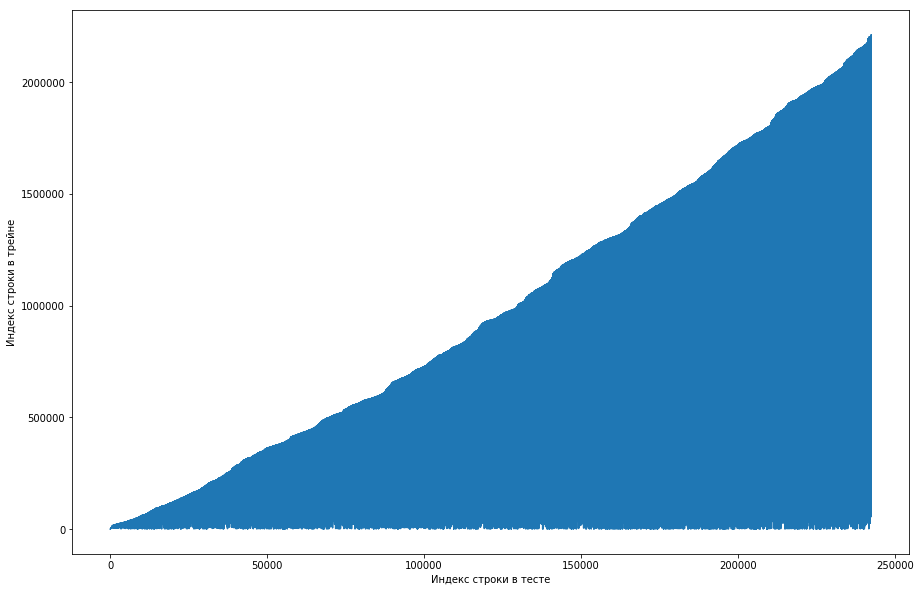
This shows that, basically, if a couple met earlier in the train, then in the test table, its position will be higher. But at the same time, there are some drops in the graph (there are actually not so many of them, but due to the resolution of the screens it seems that there is a solid triangle). Moreover, the amount of emissions roughly coincided with the expected number of units in the test. Of course, we tried to mark the emissions with units and send it to the leaderboard, but, unfortunately, it did nothing. But it still seemed to me that there might be some kind of facet (), and, as the team captain, I offered to spend more time trying to figure out how this could happen, and we still have time to train the models and generate the signs. Disclaimer: we spent a lot of time on it, but a week before the end of the competition, the organizers wrote on the forum, that only triples for the last 6 months were taken into the test dataset, but not all. Well, if you do the operations described above, but for the last 6 months, and not the whole dataset, you get a smooth monotonous curve:
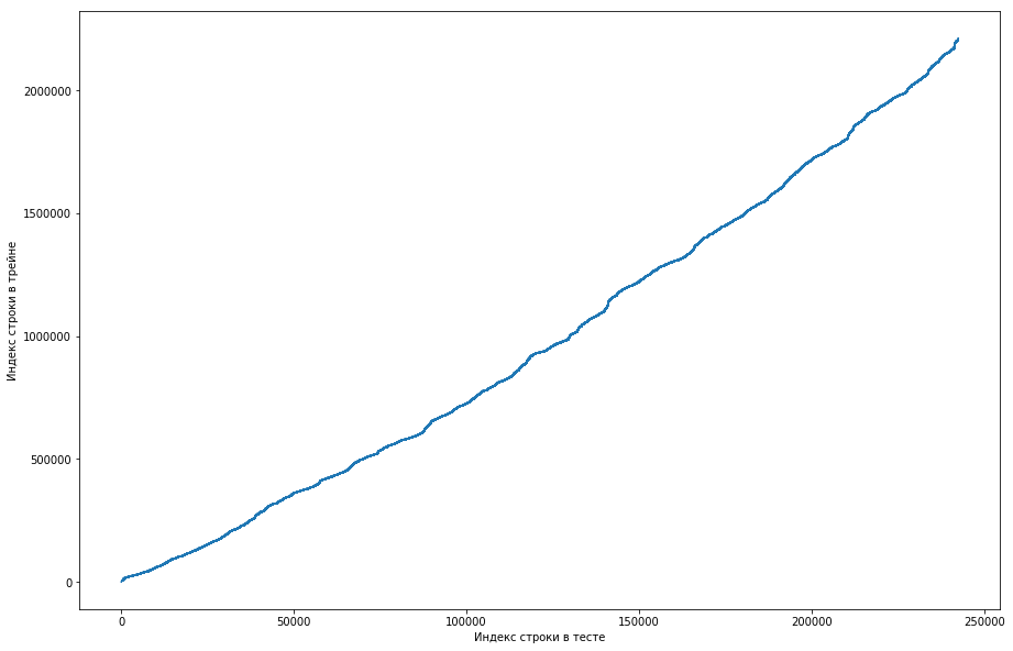
And this means that there is no face and there can not be.
Drawing up a training sample
Since in the test you need to make a prediction for triples for one week, then we divide the training data into weeks (at the same time, on average there are 20k triples “user - paper - type of transaction” on average each week). Now for any triple we can say whether she met in a particular week or not. At the same time, we already have positive triples (these are all entries from a given week in the track table), and the negative ones need to be somehow generated. There are many options for how to do this. For example, you can go through absolutely all the triples that were not on a particular week in the training dataset. It is clear that then the sample will be greatly unbalanced, and this is bad. You can first generate users in proportion to the frequency of their occurrence in dataset, and then somehow add to them in line with the action. But with this approach there will be a bunch of lines, for which it is impossible to calculate reasonable statistics, which is also bad. As we did: we took all sorts of triples that we had previously met in the train, copied, replacing buy / sell with the opposite one and condensed these two tables. It is clear that duplicates could have arisen this way (for example, if the user ever bought and sold a stock), but there were not many of them, and after deleting, a table for 500k unique triples was obtained. Well and everything, now for each week for each such three it is possible to tell, she met or not (and how many times?). and sold the stock), but there were few of them, and after deleting, a table for 500k unique triples was obtained. Well and everything, now for each week for each such three it is possible to tell, she met or not (and how many times?). and sold the stock), but there were few of them, and after deleting, a table for 500k unique triples was obtained. Well and everything, now for each week for each such three it is possible to tell, she met or not (and how many times?).
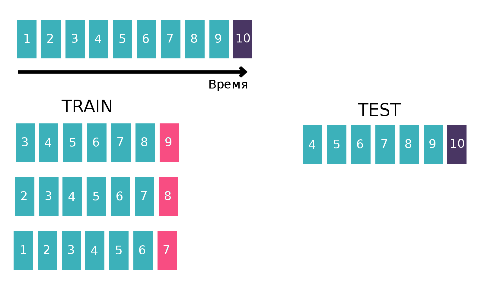
Since, in fact, we are dealing with time series — the user looks at a specific advertisement several times every week, we will build the table for training the classifier in a classic way for time series. Namely, let's take the last available week from the train, see if each of the three “customer - isin - buy or sell” met this week. This will be the target. And as a feature, we calculate various statistics, for example, for the last 6 weeks (for more information about statistics, see the “Attributes” section). Now let's forget about the existence of the last week and do everything the same, but for the penultimate week and reconstruct the resulting tables. This can be done several times, thereby increasing the “height” of the train, but at the same time, the interval over which we count the statistics naturally decreases. We repeated this operation 10 times, because if you do more, then the New Year holiday and related problems that would worsen the final quality of the model would be in the target. Explaining picture:
More information about the time series and validation of the time series can be found here .
Signs of
As I have already said, there were a lot of tables characterizing the user, share or global market conditions (rates of major currencies and some indicators). But all of them almost did not improve the quality, and the main features were the statistics counted for the customer-isin pairs and the customer-isin-buy or sell triples, for example:
- How often did a pair / triple meet in the last 1, 2, 5, 20, 100 weeks?
- Statistics on the time intervals between pairs / triples in dataset (mean, std, max, min)
- The distance in time to the first / last time the pair / troika met
- The share of each TradeStatus value for a pair / triple
- Statistics on how many times a week a pair / triple meets (mean, std, max, min)
In addition, on the last day of the competition, I read on the form that in order to sell a share, it must first be bought. This knowledge allows you to come up with many more useful signs, but for some reason, it was not obvious to me.
In the code, this all was expressed by a function of 200 lines long, which generated similar signs for each of the ten pieces of the train (for the part where the target, for example, the 7th week, we should not use the information for the 8th and 9th). Taking into account additional tables, about 300 signs were recruited. As I said, we generated 500k unique triples and took the last 10 weeks as targets, therefore the training table was “high” 500k * 10 = 5kk rows.
Some more acknowledgments were described in the second place decision.. The guys built a user / paper table, where there was a unit in each cell if the user was ever interested in the paper and zero otherwise. By calculating the cosine distance between users in this table, you can get the convergence of users among themselves. If you apply PCA to the resulting convergence table, you get a set of signs that characterize the user in some way.
Models or fight for thousands
It is worth noting that for almost three weeks no one could beat the baseline from BNP, which had a speed of 0.794 (ROC AUC) on the leaderboard, and this despite the fact that the decision “just count the number of times a pair met before” gave on the leaderboard 0.71, and some participants received and all 0.74 without the use of machine learning.
But we used machine learning, moreover, on the last day of the competition (which coincidentally coincided with the end of the session), we decided to run up
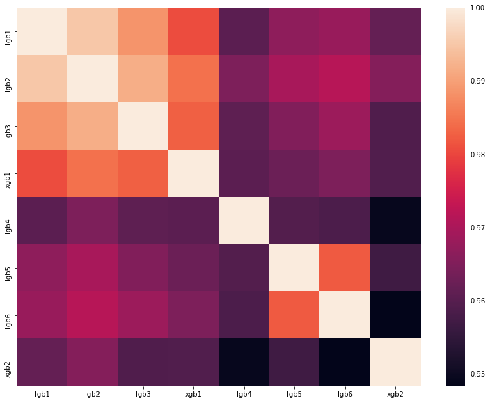
As you can see, we had a lot of rather different models, which allowed us to get 0.80204 on the leaderboard soon.
Why we will not go to France for the final stage
As a result, we showed a good result and took third place in the leaderboard. But the organizers set the following rules for the selection of finalists:
- No more than 20 top teams
- No more than 5 top teams from the country
- No more than 1 team from school
And everything would be fine if there was no other team from MIPT in the second place with 0.80272 soon. That is, we are only 0.00068 behind. It's a shame, but there's nothing you can do. Most likely, the organizers made such rules so that people from one university did not help each other in any way, but in our case, we did not know anything about the neighboring team and did not contact with it in any way.
Results
This year in September 5 teams from Russia, one from Ukraine and two teams from Germany and Finland consisting of Russian-speaking students will compete for first place in Paris. Total 8 teams of the community, which once again proves the domination of the ru-segment datasaens. And I