An example of calculating the response of a signal using the Fourier transform in the MATLAB environment
When solving problems of data transmission through the lines represented by frequency characteristics, Fourier transforms are used — transfer of signals from the time domain to the frequency domain and vice versa. The MATLAB environment has a full range of functions for solving such problems. In this paper, an example of calculating the response of a signal passing through a line, the characteristic of which is measured at frequencies that do not coincide with the data transmission frequency, is analyzed in the Matlab. I hope that this example will make it easier to understand the features of signal conversion technology in the MATLAB environment.
It is necessary to determine the change in the shape of the binary digital signal passing through the filter and the signal line. The signal is given by amplitude and transmission rate. A second-order filter, normalized to the data transfer frequency, is given by time constants. The transfer function of the signal line is represented by the measured frequency response in a complex form.
The medium used to calculate and display data - MATLAB R2015a.
The following relations were taken as an example of the initial data, published on the website www.StatEye.org for the version of the StatEye 3.0 GUI method [1, 2, 3].
The data transfer rate is bps = 10.3125 Gbit / s. The time constants of the normalized second order filter are the same; their return value is ¾ of the data transmission frequency. The signal line is represented by frequency response. The characteristic measurement was performed at channel.f = 0.006495: 0.0012475: 20 GHz. The specified number of sampling points of the Fourier transform: points = 2 ^ 13.
Figure 1 shows the data transfer, sequence and data processing results that are discussed in this paper. The transition from the time domain to the frequency domain and back is performed using the Fast Fourier Transform (FFT) algorithm.

Figure 1. Data link. The input signal is iSignal.Tx, the output signal of the filter is iSignal.Filter_out, the output of the signal line is iSignal.Rx. The characteristics presented in the diagram are discussed below.
In this paper, the main calculations are performed in the frequency domain. For this, the original signal from the time domain is transferred to the frequency domain using the Fourier transform, by multiplying the spectral characteristics of the signal, filter and signal line, the output signal of the path is found, which is transferred from the frequency domain to the time domain by the inverse Fourier transform.
The data transfer rate is two times higher than the frequency at which data transfer occurs. The maximum frequency of the measured signal line is max (channel.f) = 20 GHz. At this frequency, you can transfer data at 40 Gbit / s (as 2 * max (channel.f)).
The maximum data transfer rate that does not exceed the maximum transmission rate on the 40 Gbit / s signal line and a multiple of the transfer rate bps = 10.3125 Gbit / s is equal to fmax = 30.9375 Gbit / s, the multiplicity N = 3 (N = fmax / bps). Further, fmax is used as the limiting frequency for calculating the signal response using the Fourier transform.
Time resolution for plotting the input signal (data bit) in the time domain Ts = 1 / fmax; Ts = 3.232e-11 s. Normalized with respect to the duration of the signal, the time scale of time consists of 2 ^ 13 points (points), the scale includes the following array of points time = bps / Ts. * (1: points). The discrete single signal at a transmission rate of bps = 10.3125 Gbit / s and quantization with a period of Ts = 1 / fmax consists of three points in the range from 10 to 11 units of normalized time. A single amplitude signal can be constructed elsewhere in the timeline, but it is better to retreat from the edges in order to fully see the background and transition process of the output signal. The pulse signal (data bit) constructed using the following MATLAB commands is shown in Figure 2.

Figure 2. Input pulse signal iSignal.Tx, data bit.
The translation of the iSignal.Tx signal into the frequency domain is performed by the following FFT functions.
The FFT transform function fft builds a symmetric signal spectrum in the areas of positive and negative frequencies, the maximum frequency of which is located in the center of the spectrum (see Figure 3). The fftshift function restores the spectrum by shifting the zero frequency of the signal to the center as shown in Figure 4.
The frequency resolution of the spectrum is fs = fmax / points; The frequencies of the spectrum are in the range from -fmax / 2 to fmax / 2-fs and are equal to f = -fmax / 2: fs: fmax / 2-fs;
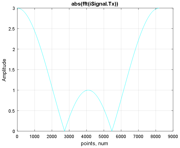
Figure 3. Amplitude characteristic of the shifted spectrum of the iSignal.Tx signal obtained using the FFT.
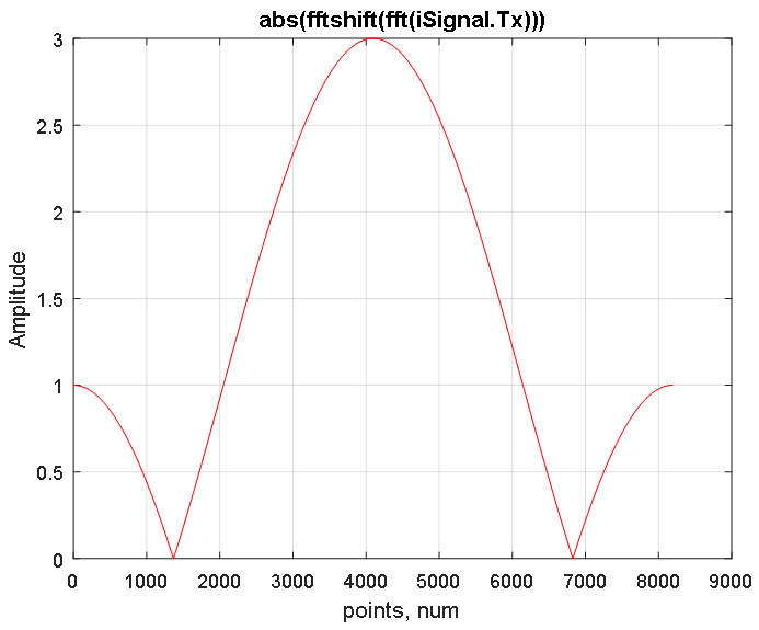
Figure 4. Amplitude response of the recovered spectrum of the iSignal.Tx signal shown in Figure 3. Presented 2 ^ 13 counts. The average count at 4097 corresponds to zero frequency. In the left part (from 1 to 4096 points) negative frequencies are located, in the right part (from 4098 to 8192 points) - the area of positive frequencies.
In this example, the transfer function of a second-order filter has the form
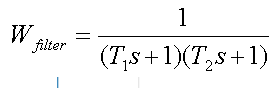
where T1 and T2 are filter time constants. The values of frequencies 1 / T1 are equal and 1 / T2 are set relative to the frequency at which data is transmitted: 1 / T1 = 1 / T2 = 0.75 * bps (bps = 10.3125 Gbit / s).
Normalized Filter Bandwidth
Operator
The amplitude-phase characteristic of the normalized filter for positive and negative frequencies normalized with respect to the signal transmission frequency is shown in Figure 5. The logarithmic amplitude-frequency characteristic of the filter is shown in Figure 6.

Figure 5. Amplitude-phase characteristic of the normalized filter
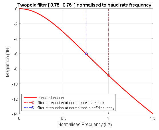
Figure 6. Logarithmic amplitude-phase frequency characteristic normalized filter. The blue dashed line shows the position of the filter frequency with a value of 0.75 from the frequency at which data is transmitted. At this frequency (1 / T1 = 1 / T2), the transmission coefficient of the second-order filter is -6 dB. The red dashed line indicates the unit frequency at which data is transmitted.
The measured amplitude and phase characteristic of the signal line includes 1599 samples in the band up to 20 GHz with a fixed step of 12.475 MHz. It contains the following frequencies: channel.f = 0.006495: 0.0012475: 20 GHz. Initially, the signal line was represented by a quadrupole characteristic. This characteristic has been transformed and is used in the example as a one-dimensional complex function.
The frequency characteristics of the signal line obtained as a result of the measurement do not coincide with the frequency spectrum of the input signal multiples of the data transmission frequency. In addition, the spectrum of the signal line contains only positive frequencies and does not contain frequencies in the region of zero. The input spectrum contains positive, zero and negative frequencies.
To convert the signal line characteristic into the transfer function — a characteristic whose frequencies coincide with the frequency spectrum of the input signal, the following steps have been performed.
1. The calculation of the amplitude characteristics of the line at zero frequency by its extrapolation. For this, the coefficients of a linear polynomial approximating the amplitude response were found by ten points of amplitude characteristic closest to the zero frequency:
The found second coefficient of the polynomial is equal to the amplitude of the characteristic at zero frequency:
2. The phase response at zero frequency is assumed to be zero.
3. Recalculation of the amplitude channel.abs and phase channel.phase characteristics of the signal line with values at zero frequency is performed on the frequency spectrum of the input signal (f = -fmax / 2: fmax / points: fmax / 2-fmax / points) with extrapolation of the characteristics in area of zero and negative frequencies:
The resulting transfer function - the amplitude-phase frequency response of the channel in the low-frequency domain is shown in Figure 7. The amplitude-frequency characteristics of the measured signal line and the calculated transfer function in the full frequency ranges are shown in Figure 8. The same characteristics in the phase space are shown in Figure 9.
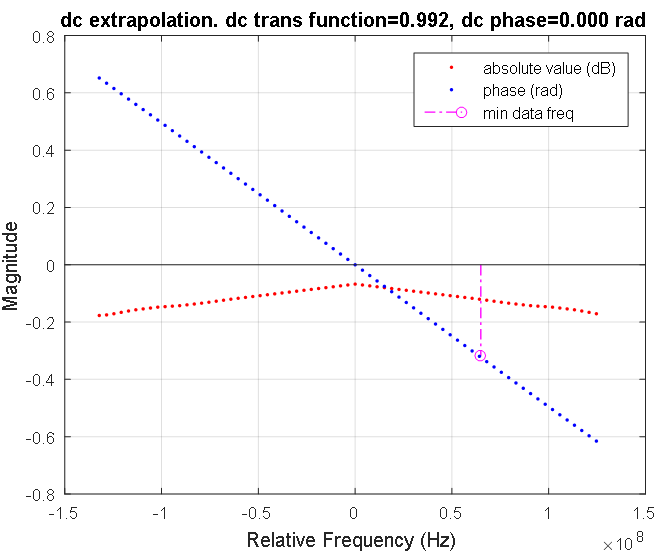
Figure 7. The transfer function of the signal line in the low frequency region. Discrete amplitude and phase characteristics are indicated by red and blue dots, respectively. The amplitude characteristic is shown in decibels, phase - in radians. The pink line indicates the lowest frequency of the measured signal line characteristic. The transmission coefficient at zero frequency is 0.992.
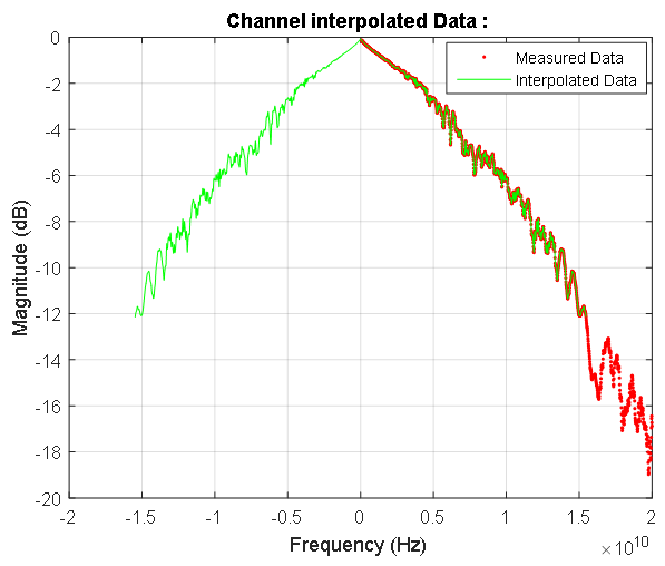
Figure 8. Amplitude-frequency characteristics of the signal line. Blue dots indicate complex measured line data. The calculated symmetric dependence of the gain of the signal line at the frequencies of the input signal spectrum is highlighted in red. In the area of zero frequencies, this characteristic is shown in Figure 7.
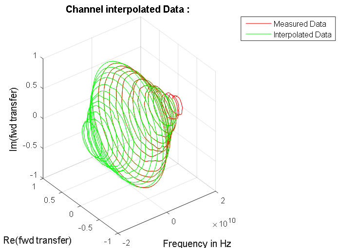
Figure 9. Amplitude-phase frequency characteristics of the measured data line and its normalized spectrum.
The reaction (response to the input action) in the frequency domain is obtained by multiplying the signal spectrum by the product of the transfer functions of the elements that associate the reaction with the input signal. In our case, the signal passes through the filter and the signal line.
To translate the signal from the frequency domain into the time domain, the inverse Fourier transform ifft is used.
The output of the filter in the time domain iSignal.Filter_out is calculated as
The output signal of the iSignal.Rx line is equal to the product of the spectrum of the input signal and the transfer functions of the filter and the signal line with the subsequent transfer of the received signal from the frequency domain to the time domain.
The filter response to the input ideal pulse and the channel response are shown in Figure 10.

Figure 10. Filter output (red graph) and data line output (green graph). The input signal of the filter - a single pulse is shown in Figure 2. The input of the signal line is the output signal of the filter.
1. IEEE802.3ap. 10.3125Gbps NRZ Simulation Results Using “StatEye” and “Signal to Interference Model” on Cascaded Channel Components. Shannon Sawyer and Charles Moore / Agilent Technologies. January 24, 2005 www.ieee802.org/3/ap/public/jan05/sawyer_01_0105.pdf
2. What is StatEye. IEEE 803.3ap Task Force. September 16, 2004 www.ieee802.org/3/ap/public/signal_adhoc/ghiasi_01_0904.pdf
3. Stat Eye / IBM Agreement. Steve Anderson. Xilinx, Inc. www.ieee802.org/3/ap/public/nov04/anderson_01_1104.pdf
The task
It is necessary to determine the change in the shape of the binary digital signal passing through the filter and the signal line. The signal is given by amplitude and transmission rate. A second-order filter, normalized to the data transfer frequency, is given by time constants. The transfer function of the signal line is represented by the measured frequency response in a complex form.
The medium used to calculate and display data - MATLAB R2015a.
The following relations were taken as an example of the initial data, published on the website www.StatEye.org for the version of the StatEye 3.0 GUI method [1, 2, 3].
The data transfer rate is bps = 10.3125 Gbit / s. The time constants of the normalized second order filter are the same; their return value is ¾ of the data transmission frequency. The signal line is represented by frequency response. The characteristic measurement was performed at channel.f = 0.006495: 0.0012475: 20 GHz. The specified number of sampling points of the Fourier transform: points = 2 ^ 13.
Figure 1 shows the data transfer, sequence and data processing results that are discussed in this paper. The transition from the time domain to the frequency domain and back is performed using the Fast Fourier Transform (FFT) algorithm.
Figure 1. Data link. The input signal is iSignal.Tx, the output signal of the filter is iSignal.Filter_out, the output of the signal line is iSignal.Rx. The characteristics presented in the diagram are discussed below.
Calculation sequence
In this paper, the main calculations are performed in the frequency domain. For this, the original signal from the time domain is transferred to the frequency domain using the Fourier transform, by multiplying the spectral characteristics of the signal, filter and signal line, the output signal of the path is found, which is transferred from the frequency domain to the time domain by the inverse Fourier transform.
The data transfer rate is two times higher than the frequency at which data transfer occurs. The maximum frequency of the measured signal line is max (channel.f) = 20 GHz. At this frequency, you can transfer data at 40 Gbit / s (as 2 * max (channel.f)).
The maximum data transfer rate that does not exceed the maximum transmission rate on the 40 Gbit / s signal line and a multiple of the transfer rate bps = 10.3125 Gbit / s is equal to fmax = 30.9375 Gbit / s, the multiplicity N = 3 (N = fmax / bps). Further, fmax is used as the limiting frequency for calculating the signal response using the Fourier transform.
The translation of the input signal in the frequency domain
Time resolution for plotting the input signal (data bit) in the time domain Ts = 1 / fmax; Ts = 3.232e-11 s. Normalized with respect to the duration of the signal, the time scale of time consists of 2 ^ 13 points (points), the scale includes the following array of points time = bps / Ts. * (1: points). The discrete single signal at a transmission rate of bps = 10.3125 Gbit / s and quantization with a period of Ts = 1 / fmax consists of three points in the range from 10 to 11 units of normalized time. A single amplitude signal can be constructed elsewhere in the timeline, but it is better to retreat from the edges in order to fully see the background and transition process of the output signal. The pulse signal (data bit) constructed using the following MATLAB commands is shown in Figure 2.
iSignal.Tx(1:size(time,2)) = 0;
t0 =    max(find(time<=10));
t1  =   max(find(time<11));
iSignal.Tx(t0:t1) = 1.0;
Figure 2. Input pulse signal iSignal.Tx, data bit.
The translation of the iSignal.Tx signal into the frequency domain is performed by the following FFT functions.
iSignal.shiftedPSD = fft(iSignal.Tx);
iSignal.PSD        = fftshift(iSignal.shiftedPSD);
The FFT transform function fft builds a symmetric signal spectrum in the areas of positive and negative frequencies, the maximum frequency of which is located in the center of the spectrum (see Figure 3). The fftshift function restores the spectrum by shifting the zero frequency of the signal to the center as shown in Figure 4.
The frequency resolution of the spectrum is fs = fmax / points; The frequencies of the spectrum are in the range from -fmax / 2 to fmax / 2-fs and are equal to f = -fmax / 2: fs: fmax / 2-fs;
Figure 3. Amplitude characteristic of the shifted spectrum of the iSignal.Tx signal obtained using the FFT.
Figure 4. Amplitude response of the recovered spectrum of the iSignal.Tx signal shown in Figure 3. Presented 2 ^ 13 counts. The average count at 4097 corresponds to zero frequency. In the left part (from 1 to 4096 points) negative frequencies are located, in the right part (from 4098 to 8192 points) - the area of positive frequencies.
The transfer function of the normalized lowpass filter
In this example, the transfer function of a second-order filter has the form
where T1 and T2 are filter time constants. The values of frequencies 1 / T1 are equal and 1 / T2 are set relative to the frequency at which data is transmitted: 1 / T1 = 1 / T2 = 0.75 * bps (bps = 10.3125 Gbit / s).
Normalized Filter Bandwidth
f_nrm =fmax/bps/points.*(-points/2:points/2-1).Operator
s = f_nrm .* j;The amplitude-phase characteristic of the normalized filter for positive and negative frequencies normalized with respect to the signal transmission frequency is shown in Figure 5. The logarithmic amplitude-frequency characteristic of the filter is shown in Figure 6.
Figure 5. Amplitude-phase characteristic of the normalized filter
Figure 6. Logarithmic amplitude-phase frequency characteristic normalized filter. The blue dashed line shows the position of the filter frequency with a value of 0.75 from the frequency at which data is transmitted. At this frequency (1 / T1 = 1 / T2), the transmission coefficient of the second-order filter is -6 dB. The red dashed line indicates the unit frequency at which data is transmitted.
Conversion of the signal line measurement results to the transfer function type
The measured amplitude and phase characteristic of the signal line includes 1599 samples in the band up to 20 GHz with a fixed step of 12.475 MHz. It contains the following frequencies: channel.f = 0.006495: 0.0012475: 20 GHz. Initially, the signal line was represented by a quadrupole characteristic. This characteristic has been transformed and is used in the example as a one-dimensional complex function.
The frequency characteristics of the signal line obtained as a result of the measurement do not coincide with the frequency spectrum of the input signal multiples of the data transmission frequency. In addition, the spectrum of the signal line contains only positive frequencies and does not contain frequencies in the region of zero. The input spectrum contains positive, zero and negative frequencies.
To convert the signal line characteristic into the transfer function — a characteristic whose frequencies coincide with the frequency spectrum of the input signal, the following steps have been performed.
1. The calculation of the amplitude characteristics of the line at zero frequency by its extrapolation. For this, the coefficients of a linear polynomial approximating the amplitude response were found by ten points of amplitude characteristic closest to the zero frequency:
[a] = polyfit(channel.f(1:10), channel.abs(1:10), 1);The found second coefficient of the polynomial is equal to the amplitude of the characteristic at zero frequency:
channel.dc = a(2);2. The phase response at zero frequency is assumed to be zero.
channel.dcPhase = 0.00;3. Recalculation of the amplitude channel.abs and phase channel.phase characteristics of the signal line with values at zero frequency is performed on the frequency spectrum of the input signal (f = -fmax / 2: fmax / points: fmax / 2-fmax / points) with extrapolation of the characteristics in area of zero and negative frequencies:
ichannel.abs   = interp1([0 channel.f], [channel.dc channel.abs],   abs(f), 'linear', 'extrap');
ichannel.phase = interp1([0 channel.f], [channel.dcPhase unwrap(channel.phase)], abs(f), 'linear', 'extrap');
ichannel.s = ichannel.abs .* exp(+j.*ichannel.phase);
ichannel.tf = real(ichannel.s) + j*imag(ichannel.s) .* sign(f);
The resulting transfer function - the amplitude-phase frequency response of the channel in the low-frequency domain is shown in Figure 7. The amplitude-frequency characteristics of the measured signal line and the calculated transfer function in the full frequency ranges are shown in Figure 8. The same characteristics in the phase space are shown in Figure 9.
Figure 7. The transfer function of the signal line in the low frequency region. Discrete amplitude and phase characteristics are indicated by red and blue dots, respectively. The amplitude characteristic is shown in decibels, phase - in radians. The pink line indicates the lowest frequency of the measured signal line characteristic. The transmission coefficient at zero frequency is 0.992.
Figure 8. Amplitude-frequency characteristics of the signal line. Blue dots indicate complex measured line data. The calculated symmetric dependence of the gain of the signal line at the frequencies of the input signal spectrum is highlighted in red. In the area of zero frequencies, this characteristic is shown in Figure 7.
Figure 9. Amplitude-phase frequency characteristics of the measured data line and its normalized spectrum.
Signal response calculation
The reaction (response to the input action) in the frequency domain is obtained by multiplying the signal spectrum by the product of the transfer functions of the elements that associate the reaction with the input signal. In our case, the signal passes through the filter and the signal line.
To translate the signal from the frequency domain into the time domain, the inverse Fourier transform ifft is used.
The output of the filter in the time domain iSignal.Filter_out is calculated as
TransFunction.PSD  = iSignal.PSD  .* Filter.PSD_Tx;
TransFunction.shiftedPSD = ifftshift(TransFunction.PSD);
iSignal.Filter_out = real(ifft(TransFunction.shiftedPSD));
The output signal of the iSignal.Rx line is equal to the product of the spectrum of the input signal and the transfer functions of the filter and the signal line with the subsequent transfer of the received signal from the frequency domain to the time domain.
TransFunction.PSD = TransFunction.PSD .* ichannel.tf;
TransFunction.shiftedPSD  = ifftshift(TransFunction.PSD);
iSignal.Rx     = real(ifft(TransFunction.shiftedPSD));
The filter response to the input ideal pulse and the channel response are shown in Figure 10.
Figure 10. Filter output (red graph) and data line output (green graph). The input signal of the filter - a single pulse is shown in Figure 2. The input of the signal line is the output signal of the filter.
Application. Used m-code MATLAB
Listing
clear all
%%%%%%%%%%%%%%%%%%%%%%%%%%%%%%%%%%%%%%%%%%%%%%% Ini data%%%%%%%%%%%%%%%%%%%%%%%%%%%%%%%%%%%%%%%%%%%%%%
bps = 1.03125e+10;
FilterParam = [0.750.75];
points                         = 2^13;
load('channel');
N = floor(max(channel.f)*2/bps);
fmax = N*bps;
%%%%%%%%%%%%%%%%%%%%%%%%%%%%%%%%%%%%%%%%%%%%%%% Signal%%%%%%%%%%%%%%%%%%%%%%%%%%%%%%%%%%%%%%%%%%%%%%% normalise all the scales for the bit rate
time        = bps/fmax .* (1:points);
iSignal.Tx(1:size(time,2)) = 0;
t0 =    max(find(time<=10));
t1  =   max(find(time<11));
iSignal.Tx(t0:t1) = 1.0;
figureplot(time(1:t1+10), iSignal.Tx(1:t1+10),'b');
hold on
plot(time(1:t1+10), iSignal.Tx(1:t1+10),'xb');
grid on
xlabel('Normalised Time, tick Ts = 1/fmax');
ylabel('Normalised Amplitude');
title(['Pulse, data bit']);
iSignal.shiftedPSD = fft(iSignal.Tx);
figureplot(abs(iSignal.shiftedPSD),'c');
grid on
xlabel('points, num');
ylabel('Amplitude');
title(['abs(fft(iSignal.Tx))']);
iSignal.PSD = fftshift(iSignal.shiftedPSD);
figureplot(abs(iSignal.PSD),'r');
grid on
xlabel('points, num');
ylabel('Amplitude');
title(['abs(fftshift(fft(iSignal.Tx)))']);
%%%%%%%%%%%%%%%%%%%%%%%%%%%%%%%%%%%%%%%%%%%%%%% Filter%%%%%%%%%%%%%%%%%%%%%%%%%%%%%%%%%%%%%%%%%%%%%%
f_nrm        =fmax/bps/points.*(-points/2:points/2-1);
s           = f_nrm .* j;
Filter_PSD = 1 ./(1 + s/FilterParam(1)) ./ (1 + s/FilterParam(2));
figure
[AX,H1,H2] = plotyy (f_nrm, abs(Filter_PSD), f_nrm, phase(Filter_PSD));
hold(AX(1));
hold(AX(2));
set(H1,'LineWidth',2);
grid(AX(2),'on');
xlabel('Normalised Frequency (Hz)');
set(get(AX(1),'Ylabel'),'String','Gain');
set(get(AX(2),'Ylabel'),'String','Phase, rad');
title(['Twopole filter [' sprintf(' %3.2f  ', FilterParam) '] normalised to baud rate frequency']);
figure
plot_handles_Filter = plot(f_nrm(points/2 + 1:points), 20*log10(abs(Filter_PSD(points/2 + 1:points))), 'r', 'linewidth', 2);
hold on
stem_handles_br = stem(1, 20*log10(abs(Filter_PSD(max(find(f_nrm < 1))))), '-.ro');
hold on
stem_handles_c = stem(FilterParam, [20*log10(abs(Filter_PSD(max(find(f_nrm < FilterParam(1)))))) 20*log10(abs(Filter_PSD(max(find(f_nrm < FilterParam(2))))))], '-.bo');
grid
legend_handles = [plot_handles_Filter, stem_handles_br(1), stem_handles_c(1)];
legend(legend_handles, 'transfer function', 'filter attenuation at normalised baud rate', 'filter attenuation at normalised cutoff frequency', 3);
xlabel('Normalised Frequency (Hz)');
ylabel('Magnitude (dB)');
title(['Twopole filter [' sprintf(' %3.2f  ', FilterParam) '] normalised to baud rate frequency']);
%%%%%%%%%%%%%%%%%%%%%%%%%%%%%%%%%%%%%%%%%%%%%%% Channel%%%%%%%%%%%%%%%%%%%%%%%%%%%%%%%%%%%%%%%%%%%%%%% create negative frequencies, convert data to complex value, taking care about negative frequency
channel.abs   = abs(channel.s);
channel.phase = angle(channel.s);
%channel.s     = channel.abs .* exp(+j.*channel.phase);
[a]        = polyfit(channel.f(1:10), channel.abs(1:10), 1);
channel.dc = a(2);
channel.dcPhase  = 0.00;
fs         = fmax/points;        % frequency step
f = -fmax/2:fs:fmax/2-fs;       % frequency matrix   % create new data structure with linearly interpolated data
ichannel.abs   = interp1([0 channel.f], [channel.dc channel.abs],   abs(f), 'linear', 'extrap');
ichannel.phase = interp1([0 channel.f], [channel.dcPhase unwrap(channel.phase)], abs(f), 'linear', 'extrap');
% correct for negative frequencies
ichannel.s = ichannel.abs .* exp(+j.*ichannel.phase);
ichannel.tf = real(ichannel.s) + j*imag(ichannel.s) .* sign(f);
figure
disp_points = 2*round(channel.f(1)/fs);
stem_handles_br = stem(channel.f(1), angle(ichannel.tf(max(find(f < channel.f(1))))), '-.mo');
hold on
plot_abs = plot(f(points/2-disp_points:points/2+disp_points), 20*log10(abs(ichannel.tf(points/2-disp_points:points/2+disp_points))), '.r', 'linewidth', 3);
hold on
plot_phase = plot(f(points/2-disp_points:points/2+disp_points), angle(ichannel.tf(points/2-disp_points:points/2+disp_points)), '.b', 'linewidth', 3);
grid
legend_handles = [plot_abs, plot_phase, stem_handles_br(1)];
legend(legend_handles, 'absolute value (dB)', 'phase (rad)', 'min data freq', 3);
xlabel('Relative Frequency (Hz)');
ylabel('Magnitude');
title(sprintf('dc extrapolation. dc trans function=%4.3f, dc phase=%4.3f rad', abs(ichannel.tf(points/2+1)), angle(ichannel.tf(points/2+1))));
figureplot(channel.f, 20*log10(channel.abs), '.r', 'linewidth', 3);
hold on
plot(f, 20*log10(ichannel.abs), 'g');
grid on
legend('Measured Data', 'Interpolated Data', 3);
xlabel('Frequency (Hz)');
ylabel('Magnitude (dB)');
title(['Chаnnel interpolated Data : ']);
figureplot3(channel.f, real(channel.s), imag(channel.s),'r');
hold on
plot3(f, real(ichannel.tf), imag(ichannel.tf),'g');
grid on
legend('Measured Data', 'Interpolated Data');
xlabel('Frequency in Hz');
ylabel('Re(fwd transfer)');
zlabel('Im(fwd transfer)');
title(['Chаnnel interpolated Data : ']);
%%%%%%%%%%%%%%%%%%%%%%%%%%%%%%%%%%%%%%%%%%%%%%% Response %%%%%%%%%%%%%%%%%%%%%%%%%%%%%%%%%%%%%%%%%%%%%%% filter Output
TransFunction.PSD  = iSignal.PSD  .* Filter_PSD;
TransFunction.shiftedPSD      = ifftshift(TransFunction.PSD);
iSignal.Filter_out                 = real(ifft(TransFunction.shiftedPSD));
% pass through channel
TransFunction.PSD = TransFunction.PSD .* ichannel.tf;
TransFunction.shiftedPSD  = ifftshift(TransFunction.PSD);
iSignal.Rx     = real(ifft(TransFunction.shiftedPSD));
figureplot(time, iSignal.Filter_out,'r');
hold on
[max_Tx, time_maxTx]     = max(iSignal.Filter_out);
[min_Tx, time_minTx]     = min(iSignal.Filter_out);
[max_Rx, time_maxRx]     = max(iSignal.Rx);
dtime_p5= round((time_maxRx - time_maxTx)*time(1) -1);
plot(time - dtime_p5, iSignal.Rx,'g');
hold on
plot(time, iSignal.Filter_out,'rx');
axis([(time_maxTx*time(1) - 3) (time_maxTx*time(1) + 5)  (min_Tx-0.15) (max_Tx+0.1)])
grid on
legend('Filter out','Rx', 2);
xlabel('Normalised Time');
ylabel('Normalised Amplitude');
title(sprintf('Transmit pulse (Tx) max= %4.3f;   Response (Rx) max (h0)= %4.3f', max(iSignal.Filter_out), max(iSignal.Rx)));
Bibliographic list
1. IEEE802.3ap. 10.3125Gbps NRZ Simulation Results Using “StatEye” and “Signal to Interference Model” on Cascaded Channel Components. Shannon Sawyer and Charles Moore / Agilent Technologies. January 24, 2005 www.ieee802.org/3/ap/public/jan05/sawyer_01_0105.pdf
2. What is StatEye. IEEE 803.3ap Task Force. September 16, 2004 www.ieee802.org/3/ap/public/signal_adhoc/ghiasi_01_0904.pdf
3. Stat Eye / IBM Agreement. Steve Anderson. Xilinx, Inc. www.ieee802.org/3/ap/public/nov04/anderson_01_1104.pdf