Optimizing the placement of virtual machines by server
Some time ago, a colleague of mine told me that the place in DC was running out, there was nowhere to put the server, but the load was growing and it was not clear what to do, and probably all the existing servers would have to be changed to more powerful ones.
At that time I was engaged in the task of compiling optimal schedules, and I thought - what if we apply optimization algorithms to increase the utilization of servers in DC? Hence the project was born, about which I want to write.
For the advanced, I’ll say at once that this article is about bin packing, and the rest, who want to know how to save up to 30% of server resources using relatively simple calculations, welcome to cat.
So, we have a DC with approximately 100 servers that host approximately 7,000 virtual machines. What is inside the virtual machines - we do not know and should not know. You need to place the virtual machines on the servers so as to perform the SLA and at the same time use the minimum number of servers.
We know:
We need to distribute virtual machines across servers so that for each of the resources on each server not to exceed the available amount of resources, and at the same time use the minimum number of servers.
This problem in the scientific literature is called the bin packing problem (how will it be in Russian?). In simple terms, this is the task of how to shove small boxes of arbitrary sizes in large boxes, and at the same time use the minimum number of large boxes. The problem in mathematics is well-known, NP-complete, exactly solved only by brute force, the cost of which combinatorially grows.
The picture below illustrates the essence of the bin packing algorithm for the one-dimensional case:

Fig. 1. Illustration of bin packing problem, non-optimal placement
In the first picture, items are somehow distributed in baskets and 3 baskets are used to place them.

Fig. 2. Illustration of bin packing problem, optimal placement.
The second picture shows the optimal distribution, for which only 2 baskets are needed.
The standard formulation of the bin packing algorithm also assumes that all baskets are the same. In our case, the servers are not the same, as they were purchased at different times and their configuration is different - different number of processor cores, memory, disk, different processor power.
A suboptimal solution can be obtained using heuristics, genetic algorithms, monte-carlo tree search and deep neural networks. We stopped at the BestFit heuristic algorithm, which converges to a solution no more than 1.7 times worse than the optimal one, and also at some variation of the genetic algorithm. Below I will give the results of their application.
But first, let's discuss what to do with time-varying metrics, such as CPU usage, disk io, network io. The easiest way is to replace the variable metric with a constant. But how to choose the value of this constant? We took the maximum value of the metric for some characteristic period (after smoothing out the outliers). A typical period in our case turned out to be a week, since the main seasonality in the load was associated with working days and weekends.
In this model, each virtual machine is allocated a bandwidth the size of the maximum consumed resource value, and each VM is described by the constants max CPU usage, RAM, disk, max disk io, max network io.
Next, we apply the algorithm for calculating the optimal packaging and get a map of the location of the VM on physical servers.
Practice shows that if you do not leave some reserve for each of the resources on the server, then with a tight placement of the VM, the server becomes overloaded. Therefore, we reserve 30% for CPU usage, 20% for RAM, 20% for disk io, 20% for network io, these limits are chosen experimentally.
We also have several types of disks (fast SSDs and slow cheap HDDs), for each of the disk types we remove the disk and disk io metrics separately, so the final model becomes somewhat more complicated and has more dimensions.
The result of the VM placement optimization is shown in the diagram:
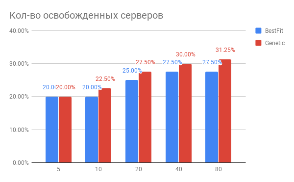
Fig. 3. The result of optimizing the placement of VM across servers.
Horizontal - the number of servers that have been optimized, vertically - the number of servers released for BestFit heuristics and for the genetic algorithm.
What conclusions can be drawn from the chart?
What other problems surfaced in practice?
Ok, we optimized VM placement. Maybe the resulting new state is very fragile with respect to increasing the load? Perhaps, servers work at a limit and any growth of loading will kill them?
We compared server utilization before and after optimization for a period of 1 week. What happened is shown in Figure 2:

Pic. 4. Changing the load on the CPU after optimizing the placement of the VM
According to CPU usage: the average CPU usage increased from 10% to only 18%. Those. we have a threefold performance margin on the CPU, while the servers will remain in the so-called "green" zone.
We collect the metrics we need in Yandex.ClickHouse (tried InfluxDB, but on our data volumes, requests with aggregation in it are executed too slowly) with a frequency of 30 seconds. From there, the task of calculating the optimal state reads the metrics, calculates the consumption maximums for them and forms the task for the calculation, which is put in a queue. As soon as the task for the calculation is performed, tests are run, verifying that the result does not go beyond the limits specified.
As we know, similar algorithms exist inside VMware vSphere and Nutanix and appear inside OpenStack (the project OpenStack Watcher).
Yes you can. In the next article, I will tell you how to pack virtual machines as tightly as possible without violating the SLA, and why you need neurons for this.
At that time I was engaged in the task of compiling optimal schedules, and I thought - what if we apply optimization algorithms to increase the utilization of servers in DC? Hence the project was born, about which I want to write.
For the advanced, I’ll say at once that this article is about bin packing, and the rest, who want to know how to save up to 30% of server resources using relatively simple calculations, welcome to cat.
So, we have a DC with approximately 100 servers that host approximately 7,000 virtual machines. What is inside the virtual machines - we do not know and should not know. You need to place the virtual machines on the servers so as to perform the SLA and at the same time use the minimum number of servers.
We know:
- server list
- the amount of resources on each server (CPU time, CPU cores, RAM, disk, disk io, network io).
- virtual machine list (VM)
- the amount of resources consumed by each virtual machine (CPU time, CPU cores, RAM, disk, disk io, network io).
- resource consumption by the host system on servers.
We need to distribute virtual machines across servers so that for each of the resources on each server not to exceed the available amount of resources, and at the same time use the minimum number of servers.
This problem in the scientific literature is called the bin packing problem (how will it be in Russian?). In simple terms, this is the task of how to shove small boxes of arbitrary sizes in large boxes, and at the same time use the minimum number of large boxes. The problem in mathematics is well-known, NP-complete, exactly solved only by brute force, the cost of which combinatorially grows.
The picture below illustrates the essence of the bin packing algorithm for the one-dimensional case:
Fig. 1. Illustration of bin packing problem, non-optimal placement
In the first picture, items are somehow distributed in baskets and 3 baskets are used to place them.
Fig. 2. Illustration of bin packing problem, optimal placement.
The second picture shows the optimal distribution, for which only 2 baskets are needed.
The standard formulation of the bin packing algorithm also assumes that all baskets are the same. In our case, the servers are not the same, as they were purchased at different times and their configuration is different - different number of processor cores, memory, disk, different processor power.
A suboptimal solution can be obtained using heuristics, genetic algorithms, monte-carlo tree search and deep neural networks. We stopped at the BestFit heuristic algorithm, which converges to a solution no more than 1.7 times worse than the optimal one, and also at some variation of the genetic algorithm. Below I will give the results of their application.
But first, let's discuss what to do with time-varying metrics, such as CPU usage, disk io, network io. The easiest way is to replace the variable metric with a constant. But how to choose the value of this constant? We took the maximum value of the metric for some characteristic period (after smoothing out the outliers). A typical period in our case turned out to be a week, since the main seasonality in the load was associated with working days and weekends.
In this model, each virtual machine is allocated a bandwidth the size of the maximum consumed resource value, and each VM is described by the constants max CPU usage, RAM, disk, max disk io, max network io.
Next, we apply the algorithm for calculating the optimal packaging and get a map of the location of the VM on physical servers.
Practice shows that if you do not leave some reserve for each of the resources on the server, then with a tight placement of the VM, the server becomes overloaded. Therefore, we reserve 30% for CPU usage, 20% for RAM, 20% for disk io, 20% for network io, these limits are chosen experimentally.
We also have several types of disks (fast SSDs and slow cheap HDDs), for each of the disk types we remove the disk and disk io metrics separately, so the final model becomes somewhat more complicated and has more dimensions.
The result of the VM placement optimization is shown in the diagram:
Fig. 3. The result of optimizing the placement of VM across servers.
Horizontal - the number of servers that have been optimized, vertically - the number of servers released for BestFit heuristics and for the genetic algorithm.
What conclusions can be drawn from the chart?
- To perform current tasks, you can use 20-30% less servers.
- The more servers you optimize at a time, the more you gain in%, with the number of servers 40 and higher, saturation occurs.
- The genetic algorithm is somewhat superior to the heuristic BestFit. If we want to further improve our results, we will dig in this direction.
What other problems surfaced in practice?
- If you want to shake up about 100 servers with 7,000 virtual machines, then the volume of migrations will be very significant, such that the whole undertaking will be impossible to implement. But if you work with groups of 20-40 servers sequentially, then the effect you get is almost the same, but the number of migrations will be many times less. And you can optimize your DC in parts.
- If you have to do live migrations, then you may be faced with a situation where the migration cannot end. This means that intensive writing to the disk and / or memory state occurs inside the VM, and the VM states between the old and new replicas do not have time to synchronize before the old replica changes its state. In this case, you need to pre-determine such VM machines and mark them as unmovable. In turn, this requires modification of optimization algorithms. What is good is the fact that the total gain practically does not depend on the number of such machines, if there are no more than 10-15% of the total number of VMs.
How does server load change after optimizing VM placement?
Ok, we optimized VM placement. Maybe the resulting new state is very fragile with respect to increasing the load? Perhaps, servers work at a limit and any growth of loading will kill them?
We compared server utilization before and after optimization for a period of 1 week. What happened is shown in Figure 2:
Pic. 4. Changing the load on the CPU after optimizing the placement of the VM
According to CPU usage: the average CPU usage increased from 10% to only 18%. Those. we have a threefold performance margin on the CPU, while the servers will remain in the so-called "green" zone.
How was it done in the software?
We collect the metrics we need in Yandex.ClickHouse (tried InfluxDB, but on our data volumes, requests with aggregation in it are executed too slowly) with a frequency of 30 seconds. From there, the task of calculating the optimal state reads the metrics, calculates the consumption maximums for them and forms the task for the calculation, which is put in a queue. As soon as the task for the calculation is performed, tests are run, verifying that the result does not go beyond the limits specified.
Has anyone already done this?
As we know, similar algorithms exist inside VMware vSphere and Nutanix and appear inside OpenStack (the project OpenStack Watcher).
Is it possible to do even better?
Yes you can. In the next article, I will tell you how to pack virtual machines as tightly as possible without violating the SLA, and why you need neurons for this.