Product recognition on the shelves using neural networks based on Keras and Tensorflow Object Detection API technologies
In the article we will talk about the use of convolutional neural networks to solve the practical business problem of recovering realogram from a photo of shelves with goods. Using the Tensorflow Object Detection API, we will train the search / localization model. Improve the quality of searching for small items in high resolution photos using a floating window and a non-maximum suppression algorithm. At Keras we sell a product classifier by brand. At the same time, we will compare approaches and results with solutions 4 years ago. All data used in the article is available for download, and the full working code is on GitHub and is designed as a tutorial.
What is a planogram? The layout of the display of goods on a specific shop equipment.
What is a realogram? The layout of the goods on a particular trade equipment existing in the store here and now.
Planogram - as it should, realogram - what we have.
Until now, in many stores, managing the rest of the goods on racks, shelves, counters, and racks is a purely manual labor. Thousands of employees check the availability of products manually, calculate the balance, compare the location with the requirements. It is expensive, and mistakes are very likely. Incorrect display or lack of goods leads to a decrease in sales.
Also, many manufacturers enter into agreements with retailers about the display of their goods. And since there are many manufacturers, the struggle for the best place on the shelf begins between them. Everyone wants his goods to be in the center opposite the buyer's eyes and occupy as large an area as possible. There is a need for continuous audit.
Thousands of merchandisers move from store to store to make sure that their company's goods are on the shelf and presented in accordance with the contract. Sometimes they are lazy: it is much more pleasant to make a report without leaving your home than to go to a point of sale. There is a need for continuous audit of auditors.
Naturally, the task of automating and simplifying this process has been solved for a long time. One of the most difficult parts was image processing: finding and recognizing products. And only relatively recently, this task has been simplified so much that for a particular case in a simplified form, its complete solution can be described in one article. This we will do.
The article contains a minimum of code (only for cases when the code is clearer than the text). The complete solution is available as an illustrated tutorial in jupyter notebooks . The article does not contain descriptions of neural network architectures, principles of operation of neurons, mathematical formulas. In the article we use them as an engineering tool, not much going into the details of its device.
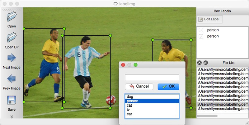
As with any data driven approach, data solutions are needed for neural network solutions. You can also collect them manually: shoot a few hundred counters and mark them using, for example, LabelImg . You can order markup, for example, on Yandex.Toloka.
We cannot disclose the details of a real project, so we will explain the technology on open data. It was too lazy to go shopping and take photos (and we would not understand us there), and the desire to independently mark up the photos found on the Internet ended after the hundredth classified object. Fortunately, quite by chance came across an archive of Grocery Dataset .
In 2014, employees of Idea Teknoloji, Istanbul, Turkey uploaded 354 photos from 40 stores made on 4 cameras. In each of these photographs, they identified a total of several thousand objects with rectangles, some of which were classified into 10 categories.
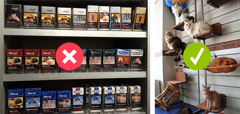
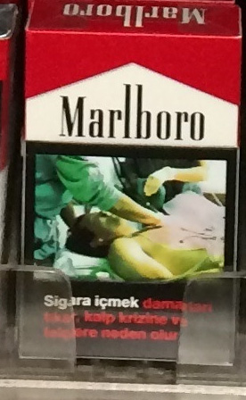
These are photos of cigarette packs. We do not promote or advertise smoking. There was simply nothing more neutral. We promise that everywhere in the article, where the situation allows, we will use photos of cats.
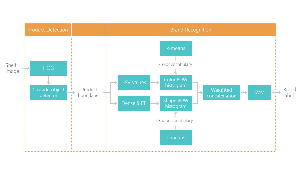
In addition to tagged photo stalls, they wrote an article on Toward Retail Product Recognition on Grocery Shelveswith the solution of the problem of localization and classification. This set a kind of benchmark: our solution with the use of new approaches should be easier and more accurate, otherwise it is not interesting. Their approach consists of a combination of algorithms:
Recently, convolutional neural networks (CNN) have revolutionized computer vision and have completely changed the approach to solving this kind of problem. Over the past few years, these technologies have become available to a wide range of developers, and such high-level APIs like Keras have significantly reduced the threshold for entry. Now almost any developer after a few days of dating can use the full power of convolutional neural networks. The article describes the use of these technologies on an example, showing how a whole cascade of algorithms can be easily replaced with just two neural networks without loss of accuracy.
We will solve the problem in steps:
The main technologies that we will use are: Tensorflow, Keras, Tensorflow Object Detection API, OpenCV. Despite the fact that both Windows and Mac OS are suitable for working with Tensorflow, we still recommend using Ubuntu. Even if you have never worked with this operating system before, its use will save you a lot of time. Installing Tensorflow for working with GPU is a topic that deserves a separate article. Fortunately, such articles already exist. For example, Installing TensorFlow on Ubuntu 16.04 with an Nvidia GPU . Some instructions from it may be outdated.
Step 1. Data preparation ( link to github )
This step, as a rule, takes much more time than the modeling itself. Fortunately, we use ready-made data that we convert into the form we need.
You can download and unpack as follows:
We obtain the following folder structure:
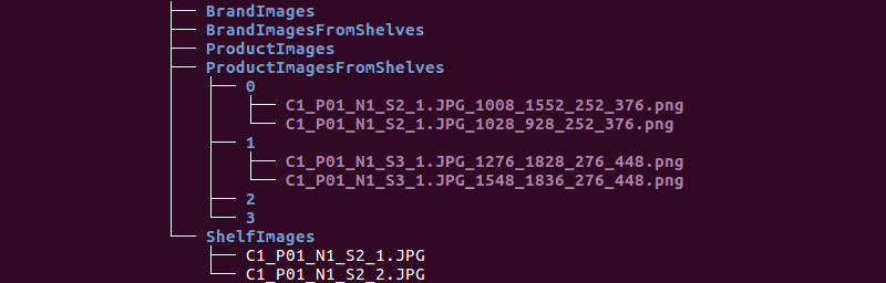
We will use information from the ShelfImages and ProductImagesFromShelves directories.
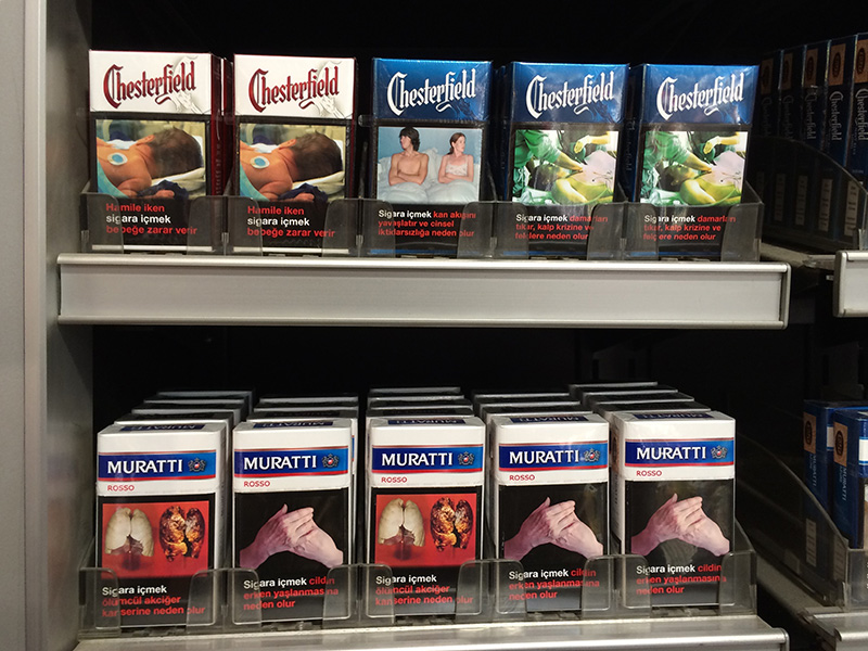
ShelfImages contains pictures of the shelves themselves. The title encoded rack ID with the ID of the snapshot. There can be several shots of one rack. For example, one photo entirely and 5 photos in parts with intersections.
File C1_P01_N1_S2_2.JPG (rack C1_P01, snapshot N1_S2_2):
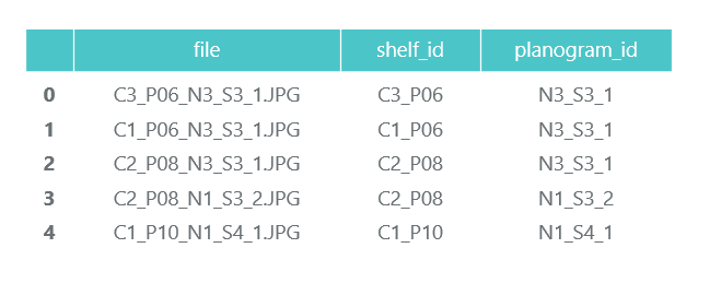
Run through all the files and collect information in pandas data frame photos_df:
ProductImagesFromShelves contains cut photos of goods from shelves in 11 subdirectories: 0 - not classified, 1 - Marlboro, 2 - Kent, etc. In order not to advertise them, we will only use category numbers without specifying names. Files in the titles contain information about the rack, the position and size of the pack on it.
File C1_P01_N1_S3_1.JPG_1276_1828_276_448.png from directory 1 (category 1, shelving C1_P01, snapshot N1_S3_1, coordinates of the upper left corner (1276, 1828), width 276, height 448):
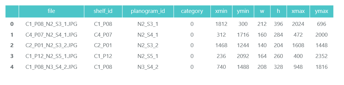
We do not need the photos of individual packs themselves (we will cut them out from the pictures of the racks), and collect information about their categories and position in pandas data frame products_df:
At the same step, we divide all our information into two sections: train for training and validation for monitoring workout. In real projects, of course, this is not worth it. And also do not trust those who do so. You must at least select another test for the final test. But even with this not very honest approach, it is important for us not to deceive ourselves too much.
As we have already noted, there can be several photos of one rack. Accordingly, the same pack can get on several pictures. Therefore, we advise you to break it not according to pictures, and especially not by packs, but by shelving. It is necessary that it did not happen that the same object, taken from different angles, turned out to be both in the train and in the validation.
We do the splitting of 70/30 (30% of the racks goes for validation, the rest is for training):
Let us ensure that at our partitioning there are enough representatives of each class both for training and for validation: The

blue color shows the number of goods in the category for validation, and the orange color for training. The situation with category 3 for validation is not very good, but in principle there are few of its representatives.
At the data preparation stage, it is important not to make a mistake, since all further work is based on its results. We still made one mistake and spent many happy hours trying to understand why the quality of the models is very mediocre. We already felt like we were the losers of the “old school” technologies, until we accidentally noticed that some of the original photos were rotated 90 degrees, and some were made upside down.
In this case, the markup is made as if the photos are oriented correctly. After a quick fix, things went much more fun.
Save our data to pkl files for use in the following steps. So we have:
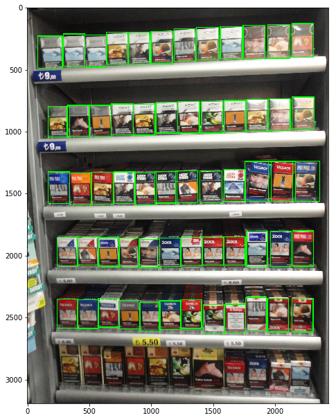
To check, let's display one rack according to our data:
Step 2. Classification by brand ( link to github )
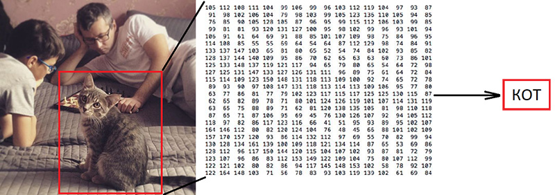
Classification of images is the main task in the field of computer vision. The problem lies in the “semantic gap”: a photograph is just a large matrix of numbers [0, 255]. For example, 800x600x3 (3 RGB channels).
Why this task is difficult:
As we have said, the authors used the data we identified 10 brands. This is an extremely simplified task, since the cigarette brands on the shelves are much larger. But everything that did not fall into these 10 categories was sent to 0 - not classified:
 "
"
Their article offers this classification algorithm with a final accuracy of 92%:

What will we do:
It sounds “volumetric”, but we just used the example of Keras “ Trains a ResNet on the CIFAR10 dataset ”, taking from it the function of creating ResNet v1.
To start the training process, it is necessary to prepare two arrays: x - photos of packs with dimension (number_packs, height, width, 3) and y - their categories with dimension (number_packs, 10). The y array contains the so-called 1-hot vectors. If the training pack category has the number 2 (from 0 to 9), then this corresponds to the vector [0, 0, 1, 0, 0, 0, 0, 0, 0, 0].
An important question is how to deal with the width and height, because all the photos were taken with different resolutions from different distances. You need to choose some fixed size, to which you can bring all our pictures of packs. This fixed size is a meta-parameter on which it depends how our neural network will train and work.
On the one hand, I want to make this size as large as possible so that not a single detail of the picture goes unnoticed. On the other hand, with our meager amount of data for training, this can lead to rapid retraining: the model will work perfectly on training data, but poorly on data for validation. We chose a size of 120x80, perhaps on a different size we would get a better result. Scaling function:
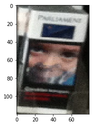
Scale and display one pack for verification. The name of the brand is read by a person with difficulty, let's see how the neural network will cope with the task of classification:
After preparing for the flag obtained in the previous step, we divide the x and y arrays into x_train / x_validation and y_train / y_validation, we get:
The data is prepared; we copy the function of the designer of the neural network of the ResNet v1 architecture from the Keras example:
We construct the model:
We have a fairly limited set of data. Therefore, in order for the model not to see the same photo every epoch during training, we use augmentation: we randomly shift the image and rotate it a little. Keras provides this set of options for this:
We start the training process.
After training and evaluation, we obtain accuracy in the region of 92%. You can have another accuracy: there is very little data, so accuracy is very much dependent on the success of the partition. At this partition, we did not get an accuracy much higher than the one mentioned in the article, but we did almost nothing ourselves and wrote little code. Moreover, we can easily add a new category, and the accuracy should (in theory) increase significantly if we prepare more data.
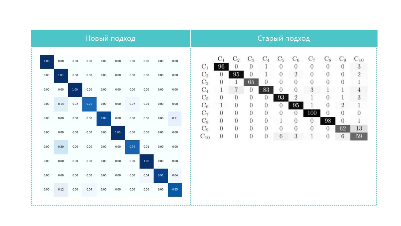
For interest, we compare confusion matrices:
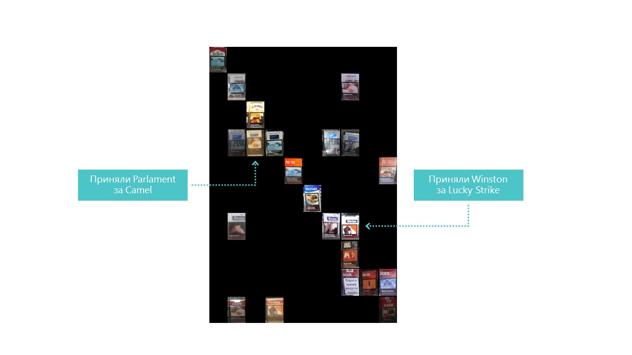
Practically all categories of our neural network are better defined, except categories 4 and 7. It is also useful to look at the brightest representatives of each confusion matrix cell:
You can also understand why Parliament was adopted for Camel, but this is why Winston was adopted for Lucky Strike - it is completely incomprehensible, they have nothing in common. This is the main problem of neural networks - the perfect opacity of what is happening inside. You can, of course, visualize some layers, but for us this visualization looks like this:
An obvious opportunity to improve the quality of recognition in our conditions is to add more photos.
So, the classifier is ready. Go to the detector.
Step 3. Search for products in the photograph ( link to github )
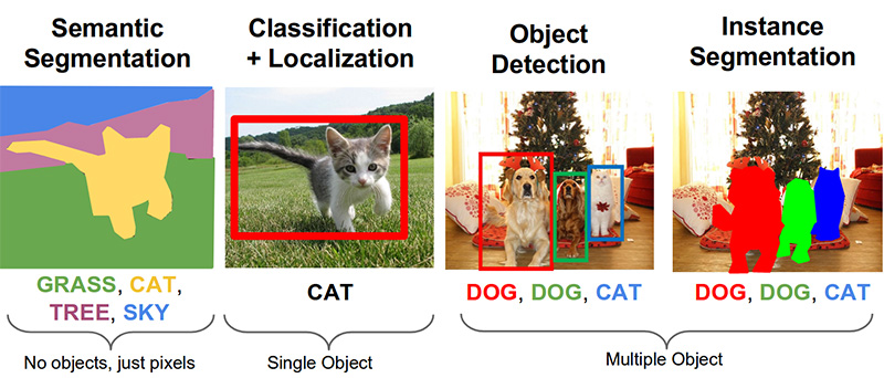
The following important tasks in the field of computer vision: semantic segmentation, localization, search for objects and segmentation of instances.
For our task, we need object detection. The 2014 article proposes an approach based on the Viola-Jones and HOG method with visual accuracy:
Thanks to the use of additional statistical constraints, their accuracy is quite good:
The object recognition problem is now successfully solved using neural networks. We will use the Tensorflow Object Detection API system and train the neural network with the SSD Mobilenet V1 architecture. Training such a model from scratch requires a lot of data and can take days, so we use a transfer training model pre-trained on COCO data.
The key concept of this approach is this. Why does the child not have to show millions of objects so that he learns to find and distinguish the ball from the cube? Because the child has 500 million years of development of the visual cortex. Evolution has made vision the largest sensory system. Nearly 50% (but this is not accurate) of the human brain neurons are responsible for image processing. Parents can only show the ball and the cube, and then several times correct the child so that he finds and distinguishes one from the other perfectly.
From a philosophical point of view (with more technical differences than a general one), transfer learning in neural networks works in a similar way. Convolutional neural networks consist of levels, each of which defines more and more complex forms: it highlights key points, combines them into lines, which in turn unites into shapes. And only at the last level from the totality of the found features determines the object.
Real world objects have a lot in common. When transfer learning, we use the already trained levels of defining basic features and train only the layers responsible for defining objects. For this we need only a couple of hundreds of photos and a couple of hours of work for an ordinary GPU. The network was originally trained on the Microsoft Common Objects in Context COCO dataset, and these are 91 categories and 2,500,000 images! Many, though not 500 million years of evolution.
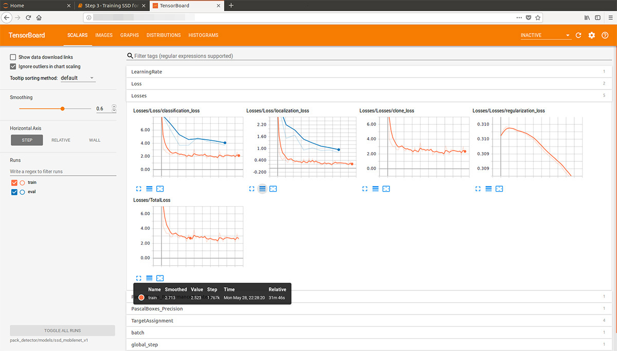
Looking ahead, this gif-animation (a bit slow, do not scroll right away) from the tensorboard visualizes the learning process. As you can see, the model begins to produce quite a high-quality result almost immediately, and further polishing continues:
The “trainer” of the Tensorflow Object Detection API system is independently able to do augmentation, cut out random parts of images for training, select “negative” examples (parts of a photo that do not contain any objects). In theory, no preprocessing of photos is needed. However, on the home computer with HDD and a small amount of RAM, he refused to work with high-resolution images: first he hung for a long time, rustled the disk, then flew out.
As a result, we squeezed the photos up to the size of 1000x1000 pixels while maintaining the aspect ratio. But since many signs are lost when compressing a large photo, at first several squares of random size were cut out of each photo of the rack and squeezed them into 1000x1000. As a result, packs in high resolution (but few) and in small (but many) were included in the training data. Again: this step is forced and, most likely, completely unnecessary, and possibly harmful.
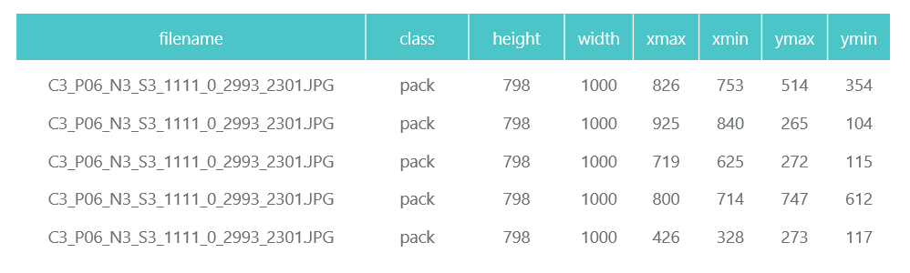
Prepared and compressed photos are saved in separate directories (eval and train), and their description (with the packs contained on them) is formed as two pandas data frame (train_df and eval_df):
The Tensorflow Object Detection API requires that input data be presented as tfrecord files. You can generate them using the utility, but we will make it code:
It remains for us to prepare a special directory and start the processes:
The structure may be different, but we find it very convenient.
The data directory contains the files we created with tfrecords (train.record and eval.record), as well as pack.pbtxt with the types of objects we are going to train the neural network for. We have only one type of designated object, so the file is very short:
The models directory (there can be many models for solving one task) in the ssd_mobilenet_v1 child directory contains settings for training in the .config file, as well as two empty directories: train and eval. In the train, the “trainer” will save the control points of the model, the “appraiser” will pick them up, run them on the data for evaluation and put them in the eval directory. Tensorboard will monitor these two directories and display information on the process.
Detailed description of the structure of configuration files, etc. can be found here and here . Instructions for installing the Tensorflow Object Detection API can be found here .
Go to the models / research / object_detection directory and download the pretrained model:
We copy there the pack_detector directory prepared by us.
First run the workout process:
We start the evaluation process. We do not have a second video card, so we run it on the processor (using the instruction CUDA_VISIBLE_DEVICES = ""). Because of this, he will be very late in the process of training, but it is not so scary:
Run the tensorboard process:
After that we can see beautiful graphs, as well as the real work of the model on the estimated data (gif at the beginning):
The training process can be stopped and resumed at any time. When we consider that the model is good enough, we save the checkpoint as an inference graph:
So, in this step, we got the inference graph, which we can use to search for objects of the packs. We proceed to its use.
Step 4. Implementing the search ( github link )
The download code inference graph and initialization is from the link above. Key search features:
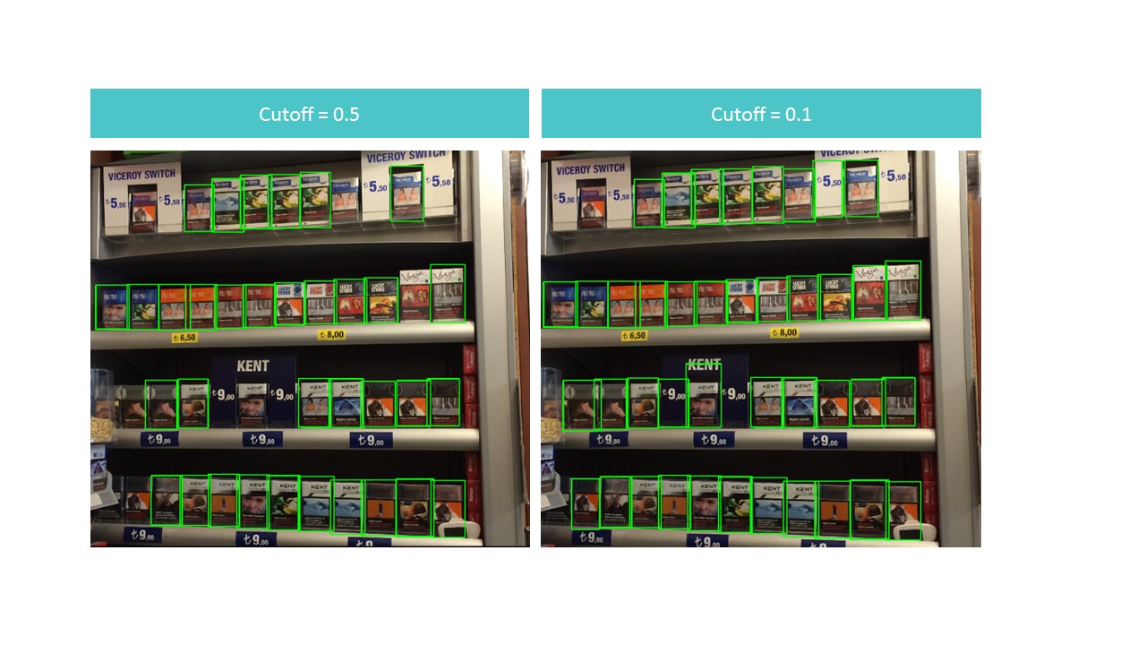
The function finds the bounding boxes (bounded boxes) for packs not on the whole photo, but on its part. Also, the function filters the detected rectangles with a low detection score (detection score) specified in the cutoff parameter.
It turns out a dilemma. On the one hand, with a high cutoff, we lose a lot of objects, on the other, with a low cutoff, we begin to find many objects that are not bundles. At the same time, we find all the same not everything and not ideal:
However, we note that if we run the function for a small piece of the photo, the recognition is almost perfect when cutoff = 0.9:
This is due to the fact that the MobileNet V1 SSD model takes the photo input 300x300. Naturally, with such compression, a lot of signs are lost.
But these signs persist if we cut a small square containing several packs. This leads to the idea of using a floating window: we run through a photo with a small rectangle and memorize everything that was found.
There is a problem: we find the same packs several times, sometimes in a very truncated version. This problem can be solved with the help of the non-maximum suppression algorithm. The idea is extremely simple: in one step we find a rectangle with a maximum recognition score (detection score), memorize it, delete all other rectangles that have an overlap area more than overlapTresh (the implementation was found on the Internet with minor changes):
The result is visually almost perfect:
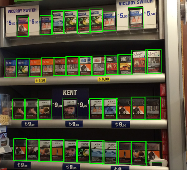
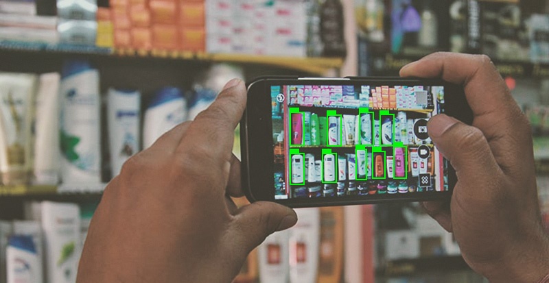
The result of working on a poor quality photo with a large number of packs:
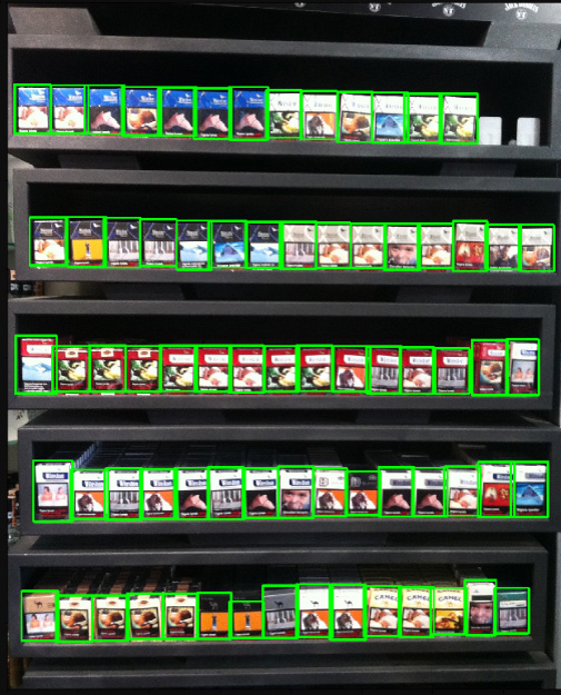
As we can see, the number of objects and the quality of the photos did not prevent us from recognizing all the packages correctly, which we wanted.
This example in our article is rather “toy”: the authors of the data have already collected them in the hope that they will have to use them for recognition. Accordingly, we chose only good pictures taken under normal lighting not at an angle, etc. Real life is much richer.
We cannot disclose the details of a real project, but here are a number of difficulties that we had to overcome:
All this drastically changes and complicates the process of data preparation, training and architecture of used neural networks, but it will not stop us.
Introduction
What is a planogram? The layout of the display of goods on a specific shop equipment.
What is a realogram? The layout of the goods on a particular trade equipment existing in the store here and now.
Planogram - as it should, realogram - what we have.
Until now, in many stores, managing the rest of the goods on racks, shelves, counters, and racks is a purely manual labor. Thousands of employees check the availability of products manually, calculate the balance, compare the location with the requirements. It is expensive, and mistakes are very likely. Incorrect display or lack of goods leads to a decrease in sales.
Also, many manufacturers enter into agreements with retailers about the display of their goods. And since there are many manufacturers, the struggle for the best place on the shelf begins between them. Everyone wants his goods to be in the center opposite the buyer's eyes and occupy as large an area as possible. There is a need for continuous audit.
Thousands of merchandisers move from store to store to make sure that their company's goods are on the shelf and presented in accordance with the contract. Sometimes they are lazy: it is much more pleasant to make a report without leaving your home than to go to a point of sale. There is a need for continuous audit of auditors.
Naturally, the task of automating and simplifying this process has been solved for a long time. One of the most difficult parts was image processing: finding and recognizing products. And only relatively recently, this task has been simplified so much that for a particular case in a simplified form, its complete solution can be described in one article. This we will do.
The article contains a minimum of code (only for cases when the code is clearer than the text). The complete solution is available as an illustrated tutorial in jupyter notebooks . The article does not contain descriptions of neural network architectures, principles of operation of neurons, mathematical formulas. In the article we use them as an engineering tool, not much going into the details of its device.
Data and approach
As with any data driven approach, data solutions are needed for neural network solutions. You can also collect them manually: shoot a few hundred counters and mark them using, for example, LabelImg . You can order markup, for example, on Yandex.Toloka.
We cannot disclose the details of a real project, so we will explain the technology on open data. It was too lazy to go shopping and take photos (and we would not understand us there), and the desire to independently mark up the photos found on the Internet ended after the hundredth classified object. Fortunately, quite by chance came across an archive of Grocery Dataset .
In 2014, employees of Idea Teknoloji, Istanbul, Turkey uploaded 354 photos from 40 stores made on 4 cameras. In each of these photographs, they identified a total of several thousand objects with rectangles, some of which were classified into 10 categories.
These are photos of cigarette packs. We do not promote or advertise smoking. There was simply nothing more neutral. We promise that everywhere in the article, where the situation allows, we will use photos of cats.
In addition to tagged photo stalls, they wrote an article on Toward Retail Product Recognition on Grocery Shelveswith the solution of the problem of localization and classification. This set a kind of benchmark: our solution with the use of new approaches should be easier and more accurate, otherwise it is not interesting. Their approach consists of a combination of algorithms:
Recently, convolutional neural networks (CNN) have revolutionized computer vision and have completely changed the approach to solving this kind of problem. Over the past few years, these technologies have become available to a wide range of developers, and such high-level APIs like Keras have significantly reduced the threshold for entry. Now almost any developer after a few days of dating can use the full power of convolutional neural networks. The article describes the use of these technologies on an example, showing how a whole cascade of algorithms can be easily replaced with just two neural networks without loss of accuracy.
We will solve the problem in steps:
- Data preparation. We will download archives and transform it into a convenient for work look.
- Brand classification. We solve the problem of classification using a neural network.
- Search for products in the photo. We will train the neural network to search for goods.
- The implementation of the search. Improve the quality of detection using a floating window and a non-maximum suppression algorithm.
- Conclusion Let us briefly explain why real life is much more complicated than this example.
Technology
The main technologies that we will use are: Tensorflow, Keras, Tensorflow Object Detection API, OpenCV. Despite the fact that both Windows and Mac OS are suitable for working with Tensorflow, we still recommend using Ubuntu. Even if you have never worked with this operating system before, its use will save you a lot of time. Installing Tensorflow for working with GPU is a topic that deserves a separate article. Fortunately, such articles already exist. For example, Installing TensorFlow on Ubuntu 16.04 with an Nvidia GPU . Some instructions from it may be outdated.
Step 1. Data preparation ( link to github )
This step, as a rule, takes much more time than the modeling itself. Fortunately, we use ready-made data that we convert into the form we need.
You can download and unpack as follows:
wget https://github.com/gulvarol/grocerydataset/releases/download/1.0/GroceryDataset_part1.tar.gz
wget https://github.com/gulvarol/grocerydataset/releases/download/1.0/GroceryDataset_part2.tar.gz
tar -xvzf GroceryDataset_part1.tar.gz
tar -xvzf GroceryDataset_part2.tar.gz
We obtain the following folder structure:
We will use information from the ShelfImages and ProductImagesFromShelves directories.
ShelfImages contains pictures of the shelves themselves. The title encoded rack ID with the ID of the snapshot. There can be several shots of one rack. For example, one photo entirely and 5 photos in parts with intersections.
File C1_P01_N1_S2_2.JPG (rack C1_P01, snapshot N1_S2_2):
Run through all the files and collect information in pandas data frame photos_df:
ProductImagesFromShelves contains cut photos of goods from shelves in 11 subdirectories: 0 - not classified, 1 - Marlboro, 2 - Kent, etc. In order not to advertise them, we will only use category numbers without specifying names. Files in the titles contain information about the rack, the position and size of the pack on it.
File C1_P01_N1_S3_1.JPG_1276_1828_276_448.png from directory 1 (category 1, shelving C1_P01, snapshot N1_S3_1, coordinates of the upper left corner (1276, 1828), width 276, height 448):
We do not need the photos of individual packs themselves (we will cut them out from the pictures of the racks), and collect information about their categories and position in pandas data frame products_df:
At the same step, we divide all our information into two sections: train for training and validation for monitoring workout. In real projects, of course, this is not worth it. And also do not trust those who do so. You must at least select another test for the final test. But even with this not very honest approach, it is important for us not to deceive ourselves too much.
As we have already noted, there can be several photos of one rack. Accordingly, the same pack can get on several pictures. Therefore, we advise you to break it not according to pictures, and especially not by packs, but by shelving. It is necessary that it did not happen that the same object, taken from different angles, turned out to be both in the train and in the validation.
We do the splitting of 70/30 (30% of the racks goes for validation, the rest is for training):
# get distinct shelves
shelves = list(set(photos_df['shelf_id'].values))
# use train_test_split from sklearn
shelves_train, shelves_validation, _, _ = train_test_split(
    shelves, shelves, test_size=0.3, random_state=6)
# mark all records in data frames with is_train flagdefis_train(shelf_id):return shelf_id in shelves_train
photos_df['is_train'] = photos_df.shelf_id.apply(is_train)
products_df['is_train'] = products_df.shelf_id.apply(is_train)
Let us ensure that at our partitioning there are enough representatives of each class both for training and for validation: The
blue color shows the number of goods in the category for validation, and the orange color for training. The situation with category 3 for validation is not very good, but in principle there are few of its representatives.
At the data preparation stage, it is important not to make a mistake, since all further work is based on its results. We still made one mistake and spent many happy hours trying to understand why the quality of the models is very mediocre. We already felt like we were the losers of the “old school” technologies, until we accidentally noticed that some of the original photos were rotated 90 degrees, and some were made upside down.
In this case, the markup is made as if the photos are oriented correctly. After a quick fix, things went much more fun.
Save our data to pkl files for use in the following steps. So we have:
- Directory of photos of racks and their parts with packs,
- A data frame with a description of each rack, indicating whether it is intended for training,
- A data frame with information on all goods on the racks, indicating their position, size, category, and whether they are intended for training.
To check, let's display one rack according to our data:
# function to display shelf photo with rectangled productsdefdraw_shelf_photo(file):
    file_products_df = products_df[products_df.file == file]
    coordinates = file_products_df[['xmin', 'ymin', 'xmax', 'ymax']].values
    im = cv2.imread(f'{shelf_images}{file}')
    im = cv2.cvtColor(im, cv2.COLOR_BGR2RGB)
    for xmin, ymin, xmax, ymax in coordinates:
        cv2.rectangle(im, (xmin, ymin), (xmax, ymax), (0, 255, 0), 5)
    plt.imshow(im)
# draw one photo to check our data
fig = plt.gcf()
fig.set_size_inches(18.5, 10.5)
draw_shelf_photo('C3_P07_N1_S6_1.JPG')
Step 2. Classification by brand ( link to github )
Classification of images is the main task in the field of computer vision. The problem lies in the “semantic gap”: a photograph is just a large matrix of numbers [0, 255]. For example, 800x600x3 (3 RGB channels).
Why this task is difficult:
As we have said, the authors used the data we identified 10 brands. This is an extremely simplified task, since the cigarette brands on the shelves are much larger. But everything that did not fall into these 10 categories was sent to 0 - not classified:
" Their article offers this classification algorithm with a final accuracy of 92%:
What will we do:
- Prepare data for training
- We will train the convolutional neural network with the ResNet v1 architecture,
- Check on photos for validation.
It sounds “volumetric”, but we just used the example of Keras “ Trains a ResNet on the CIFAR10 dataset ”, taking from it the function of creating ResNet v1.
To start the training process, it is necessary to prepare two arrays: x - photos of packs with dimension (number_packs, height, width, 3) and y - their categories with dimension (number_packs, 10). The y array contains the so-called 1-hot vectors. If the training pack category has the number 2 (from 0 to 9), then this corresponds to the vector [0, 0, 1, 0, 0, 0, 0, 0, 0, 0].
An important question is how to deal with the width and height, because all the photos were taken with different resolutions from different distances. You need to choose some fixed size, to which you can bring all our pictures of packs. This fixed size is a meta-parameter on which it depends how our neural network will train and work.
On the one hand, I want to make this size as large as possible so that not a single detail of the picture goes unnoticed. On the other hand, with our meager amount of data for training, this can lead to rapid retraining: the model will work perfectly on training data, but poorly on data for validation. We chose a size of 120x80, perhaps on a different size we would get a better result. Scaling function:
# resize pack to fixed size SHAPE_WIDTH x SHAPE_HEIGHTdefresize_pack(pack):
    fx_ratio = SHAPE_WIDTH / pack.shape[1]
    fy_ratio = SHAPE_HEIGHT / pack.shape[0]
    pack = cv2.resize(pack, (0, 0), fx=fx_ratio, fy=fy_ratio)
    return pack[0:SHAPE_HEIGHT, 0:SHAPE_WIDTH]
Scale and display one pack for verification. The name of the brand is read by a person with difficulty, let's see how the neural network will cope with the task of classification:
After preparing for the flag obtained in the previous step, we divide the x and y arrays into x_train / x_validation and y_train / y_validation, we get:
x_train shape: (1969, 120, 80, 3)
y_train shape: (1969, 10)
1969 train samples
775 validation samples
The data is prepared; we copy the function of the designer of the neural network of the ResNet v1 architecture from the Keras example:
defresnet_v1(input_shape, depth, num_classes=10):
    …
We construct the model:
model = resnet_v1(input_shape=x_train.shape[1:], depth=depth, num_classes=num_classes)
model.compile(loss='categorical_crossentropy',
              optimizer=Adam(lr=lr_schedule(0)), metrics=['accuracy'])
We have a fairly limited set of data. Therefore, in order for the model not to see the same photo every epoch during training, we use augmentation: we randomly shift the image and rotate it a little. Keras provides this set of options for this:
# This will do preprocessing and realtime data augmentation:
datagen = ImageDataGenerator(
    featurewise_center=False,  # set input mean to 0 over the dataset
    samplewise_center=False,  # set each sample mean to 0
    featurewise_std_normalization=False,  # divide inputs by std of the dataset
    samplewise_std_normalization=False,  # divide each input by its std
    zca_whitening=False,  # apply ZCA whitening
    rotation_range=5,  # randomly rotate images in the range (degrees, 0 to 180)
    width_shift_range=0.1,  # randomly shift images horizontally (fraction of total width)
    height_shift_range=0.1,  # randomly shift images vertically (fraction of total height)
    horizontal_flip=False,  # randomly flip images
    vertical_flip=False)  # randomly flip images
datagen.fit(x_train)
We start the training process.
# let's run training process, 20 epochs is enough
batch_size = 50
epochs = 15
model.fit_generator(datagen.flow(x_train, y_train, batch_size=batch_size),
                    validation_data=(x_validation, y_validation),
                    epochs=epochs, verbose=1, workers=4,
                    callbacks=[LearningRateScheduler(lr_schedule)])
After training and evaluation, we obtain accuracy in the region of 92%. You can have another accuracy: there is very little data, so accuracy is very much dependent on the success of the partition. At this partition, we did not get an accuracy much higher than the one mentioned in the article, but we did almost nothing ourselves and wrote little code. Moreover, we can easily add a new category, and the accuracy should (in theory) increase significantly if we prepare more data.
For interest, we compare confusion matrices:
Practically all categories of our neural network are better defined, except categories 4 and 7. It is also useful to look at the brightest representatives of each confusion matrix cell:
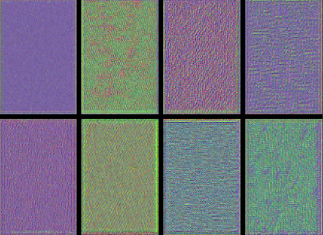
You can also understand why Parliament was adopted for Camel, but this is why Winston was adopted for Lucky Strike - it is completely incomprehensible, they have nothing in common. This is the main problem of neural networks - the perfect opacity of what is happening inside. You can, of course, visualize some layers, but for us this visualization looks like this:
An obvious opportunity to improve the quality of recognition in our conditions is to add more photos.
So, the classifier is ready. Go to the detector.
Step 3. Search for products in the photograph ( link to github )
The following important tasks in the field of computer vision: semantic segmentation, localization, search for objects and segmentation of instances.
For our task, we need object detection. The 2014 article proposes an approach based on the Viola-Jones and HOG method with visual accuracy:
Thanks to the use of additional statistical constraints, their accuracy is quite good:
The object recognition problem is now successfully solved using neural networks. We will use the Tensorflow Object Detection API system and train the neural network with the SSD Mobilenet V1 architecture. Training such a model from scratch requires a lot of data and can take days, so we use a transfer training model pre-trained on COCO data.
The key concept of this approach is this. Why does the child not have to show millions of objects so that he learns to find and distinguish the ball from the cube? Because the child has 500 million years of development of the visual cortex. Evolution has made vision the largest sensory system. Nearly 50% (but this is not accurate) of the human brain neurons are responsible for image processing. Parents can only show the ball and the cube, and then several times correct the child so that he finds and distinguishes one from the other perfectly.
From a philosophical point of view (with more technical differences than a general one), transfer learning in neural networks works in a similar way. Convolutional neural networks consist of levels, each of which defines more and more complex forms: it highlights key points, combines them into lines, which in turn unites into shapes. And only at the last level from the totality of the found features determines the object.
Real world objects have a lot in common. When transfer learning, we use the already trained levels of defining basic features and train only the layers responsible for defining objects. For this we need only a couple of hundreds of photos and a couple of hours of work for an ordinary GPU. The network was originally trained on the Microsoft Common Objects in Context COCO dataset, and these are 91 categories and 2,500,000 images! Many, though not 500 million years of evolution.
Looking ahead, this gif-animation (a bit slow, do not scroll right away) from the tensorboard visualizes the learning process. As you can see, the model begins to produce quite a high-quality result almost immediately, and further polishing continues:
The “trainer” of the Tensorflow Object Detection API system is independently able to do augmentation, cut out random parts of images for training, select “negative” examples (parts of a photo that do not contain any objects). In theory, no preprocessing of photos is needed. However, on the home computer with HDD and a small amount of RAM, he refused to work with high-resolution images: first he hung for a long time, rustled the disk, then flew out.
As a result, we squeezed the photos up to the size of 1000x1000 pixels while maintaining the aspect ratio. But since many signs are lost when compressing a large photo, at first several squares of random size were cut out of each photo of the rack and squeezed them into 1000x1000. As a result, packs in high resolution (but few) and in small (but many) were included in the training data. Again: this step is forced and, most likely, completely unnecessary, and possibly harmful.
Prepared and compressed photos are saved in separate directories (eval and train), and their description (with the packs contained on them) is formed as two pandas data frame (train_df and eval_df):
The Tensorflow Object Detection API requires that input data be presented as tfrecord files. You can generate them using the utility, but we will make it code:
defclass_text_to_int(row_label):
    if row_label == 'pack':
        return1
    else:
        Nonedefsplit(df, group):
    data = namedtuple('data', ['filename', 'object'])
    gb = df.groupby(group)
    return [data(filename, gb.get_group(x))
            for filename, x in zip(gb.groups.keys(), gb.groups)]
defcreate_tf_example(group, path):
    with tf.gfile.GFile(os.path.join(path, '{}'.format(group.filename)), 'rb') as fid:
        encoded_jpg = fid.read()
    encoded_jpg_io = io.BytesIO(encoded_jpg)
    image = Image.open(encoded_jpg_io)
    width, height = image.size
    filename = group.filename.encode('utf8')
    image_format = b'jpg'
    xmins = []
    xmaxs = []
    ymins = []
    ymaxs = []
    classes_text = []
    classes = []
    for index, row in group.object.iterrows():
        xmins.append(row['xmin'] / width)
        xmaxs.append(row['xmax'] / width)
        ymins.append(row['ymin'] / height)
        ymaxs.append(row['ymax'] / height)
        classes_text.append(row['class'].encode('utf8'))
        classes.append(class_text_to_int(row['class']))
    tf_example = tf.train.Example(features=tf.train.Features(feature={
        'image/height': dataset_util.int64_feature(height),
        'image/width': dataset_util.int64_feature(width),
        'image/filename': dataset_util.bytes_feature(filename),
        'image/source_id': dataset_util.bytes_feature(filename),
        'image/encoded': dataset_util.bytes_feature(encoded_jpg),
        'image/format': dataset_util.bytes_feature(image_format),
        'image/object/bbox/xmin': dataset_util.float_list_feature(xmins),
        'image/object/bbox/xmax': dataset_util.float_list_feature(xmaxs),
        'image/object/bbox/ymin': dataset_util.float_list_feature(ymins),
        'image/object/bbox/ymax': dataset_util.float_list_feature(ymaxs),
        'image/object/class/text': dataset_util.bytes_list_feature(classes_text),
        'image/object/class/label': dataset_util.int64_list_feature(classes),
    }))
    return tf_example
defconvert_to_tf_records(images_path, examples, dst_file):
    writer = tf.python_io.TFRecordWriter(dst_file)
    grouped = split(examples, 'filename')
    for group in grouped:
        tf_example = create_tf_example(group, images_path)
        writer.write(tf_example.SerializeToString())
    writer.close()
convert_to_tf_records(f'{cropped_path}train/', train_df, f'{detector_data_path}train.record')
convert_to_tf_records(f'{cropped_path}eval/', eval_df, f'{detector_data_path}eval.record')
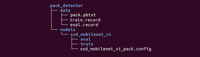
It remains for us to prepare a special directory and start the processes:
The structure may be different, but we find it very convenient.
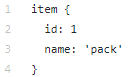
The data directory contains the files we created with tfrecords (train.record and eval.record), as well as pack.pbtxt with the types of objects we are going to train the neural network for. We have only one type of designated object, so the file is very short:
The models directory (there can be many models for solving one task) in the ssd_mobilenet_v1 child directory contains settings for training in the .config file, as well as two empty directories: train and eval. In the train, the “trainer” will save the control points of the model, the “appraiser” will pick them up, run them on the data for evaluation and put them in the eval directory. Tensorboard will monitor these two directories and display information on the process.
Detailed description of the structure of configuration files, etc. can be found here and here . Instructions for installing the Tensorflow Object Detection API can be found here .
Go to the models / research / object_detection directory and download the pretrained model:
wget http://download.tensorflow.org/models/object_detection/ssd_mobilenet_v1_coco_2017_11_17.tar.gz
tar -xvzf ssd_mobilenet_v1_coco_2017_11_17.tar.gz
We copy there the pack_detector directory prepared by us.
First run the workout process:
python3 train.py --logtostderr \
    --train_dir=pack_detector/models/ssd_mobilenet_v1/train/ \
    --pipeline_config_path=pack_detector/models/ssd_mobilenet_v1/ssd_mobilenet_v1_pack.config
We start the evaluation process. We do not have a second video card, so we run it on the processor (using the instruction CUDA_VISIBLE_DEVICES = ""). Because of this, he will be very late in the process of training, but it is not so scary:
CUDA_VISIBLE_DEVICES="" python3 eval.py \
    --logtostderr \
    --checkpoint_dir=pack_detector/models/ssd_mobilenet_v1/train \
    --pipeline_config_path=pack_detector/models/ssd_mobilenet_v1/ssd_mobilenet_v1_pack.config \
    --eval_dir=pack_detector/models/ssd_mobilenet_v1/eval
Run the tensorboard process:
tensorboard --logdir=pack_detector/models/ssd_mobilenet_v1After that we can see beautiful graphs, as well as the real work of the model on the estimated data (gif at the beginning):
The training process can be stopped and resumed at any time. When we consider that the model is good enough, we save the checkpoint as an inference graph:
python3 export_inference_graph.py \
    --input_type image_tensor \
    --pipeline_config_path pack_detector/models/ssd_mobilenet_v1/ssd_mobilenet_v1_pack.config \
    --trained_checkpoint_prefix pack_detector/models/ssd_mobilenet_v1/train/model.ckpt-13756 \
    --output_directory pack_detector/models/ssd_mobilenet_v1/pack_detector_2018_06_03
So, in this step, we got the inference graph, which we can use to search for objects of the packs. We proceed to its use.
Step 4. Implementing the search ( github link )
The download code inference graph and initialization is from the link above. Key search features:
# let's write function that executes detectiondefrun_inference_for_single_image(image, image_tensor, sess, tensor_dict):
    # Run inference
    expanded_dims = np.expand_dims(image, 0)
    output_dict = sess.run(tensor_dict, feed_dict={image_tensor: expanded_dims})
    # all outputs are float32 numpy arrays, so convert types as appropriate
    output_dict['num_detections'] = int(output_dict['num_detections'][0])
    output_dict['detection_classes'] = output_dict['detection_classes'][0].astype(np.uint8)
    output_dict['detection_boxes'] = output_dict['detection_boxes'][0]
    output_dict['detection_scores'] = output_dict['detection_scores'][0]
    return output_dict
# it is useful to be able to run inference not only on the whole image,# but also on its parts# cutoff - minimum detection score needed to take boxdefrun_inference_for_image_part(image_tensor, sess, tensor_dict,
                                 image, cutoff, ax0, ay0, ax1, ay1):
    boxes = []
    im = image[ay0:ay1, ax0:ax1]
    h, w, c = im.shape
    output_dict = run_inference_for_single_image(im, image_tensor, sess, tensor_dict)
    for i in range(100):
        if output_dict['detection_scores'][i] < cutoff:
            break
        y0, x0, y1, x1, score = *output_dict['detection_boxes'][i], \
                                output_dict['detection_scores'][i]
        x0, y0, x1, y1, score = int(x0*w), int(y0*h), \
                                int(x1*w), int(y1*h), \
                                int(score * 100)
        boxes.append((x0+ax0, y0+ay0, x1+ax0, y1+ay0, score))
    return boxes
The function finds the bounding boxes (bounded boxes) for packs not on the whole photo, but on its part. Also, the function filters the detected rectangles with a low detection score (detection score) specified in the cutoff parameter.
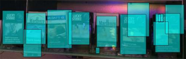
It turns out a dilemma. On the one hand, with a high cutoff, we lose a lot of objects, on the other, with a low cutoff, we begin to find many objects that are not bundles. At the same time, we find all the same not everything and not ideal:
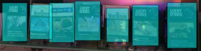
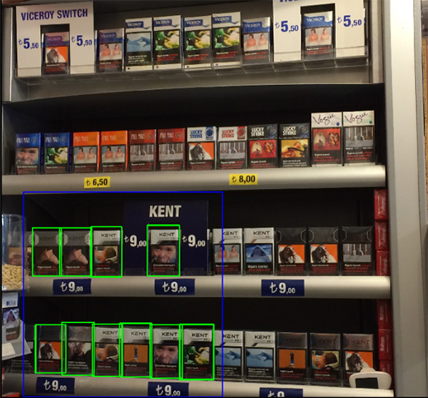
However, we note that if we run the function for a small piece of the photo, the recognition is almost perfect when cutoff = 0.9:
This is due to the fact that the MobileNet V1 SSD model takes the photo input 300x300. Naturally, with such compression, a lot of signs are lost.
But these signs persist if we cut a small square containing several packs. This leads to the idea of using a floating window: we run through a photo with a small rectangle and memorize everything that was found.
There is a problem: we find the same packs several times, sometimes in a very truncated version. This problem can be solved with the help of the non-maximum suppression algorithm. The idea is extremely simple: in one step we find a rectangle with a maximum recognition score (detection score), memorize it, delete all other rectangles that have an overlap area more than overlapTresh (the implementation was found on the Internet with minor changes):
# function for non-maximum suppressiondefnon_max_suppression(boxes, overlapThresh):
    if len(boxes) == 0:
        return np.array([]).astype("int")
    if boxes.dtype.kind == "i":
        boxes = boxes.astype("float")
    pick = []
    x1 = boxes[:,0]
    y1 = boxes[:,1]
    x2 = boxes[:,2]
    y2 = boxes[:,3]
    sc = boxes[:,4]
    area = (x2 - x1 + 1) * (y2 - y1 + 1)
    idxs = np.argsort(sc)
    while len(idxs) > 0:
        last = len(idxs) - 1
        i = idxs[last]
        pick.append(i)
        xx1 = np.maximum(x1[i], x1[idxs[:last]])
        yy1 = np.maximum(y1[i], y1[idxs[:last]])
        xx2 = np.minimum(x2[i], x2[idxs[:last]])
        yy2 = np.minimum(y2[i], y2[idxs[:last]])
        w = np.maximum(0, xx2 - xx1 + 1)
        h = np.maximum(0, yy2 - yy1 + 1)
        #todo fix overlap-contains...
        overlap = (w * h) / area[idxs[:last]]

        idxs = np.delete(idxs, np.concatenate(([last],
            np.where(overlap > overlapThresh)[0])))

    return boxes[pick].astype("int")
The result is visually almost perfect:
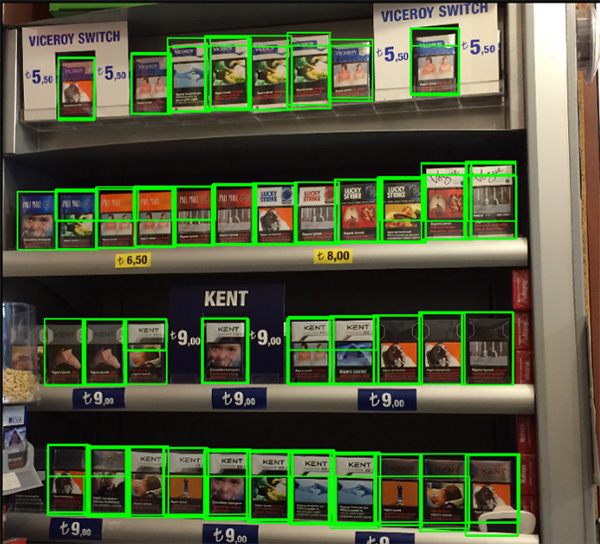
The result of working on a poor quality photo with a large number of packs:
As we can see, the number of objects and the quality of the photos did not prevent us from recognizing all the packages correctly, which we wanted.
Conclusion
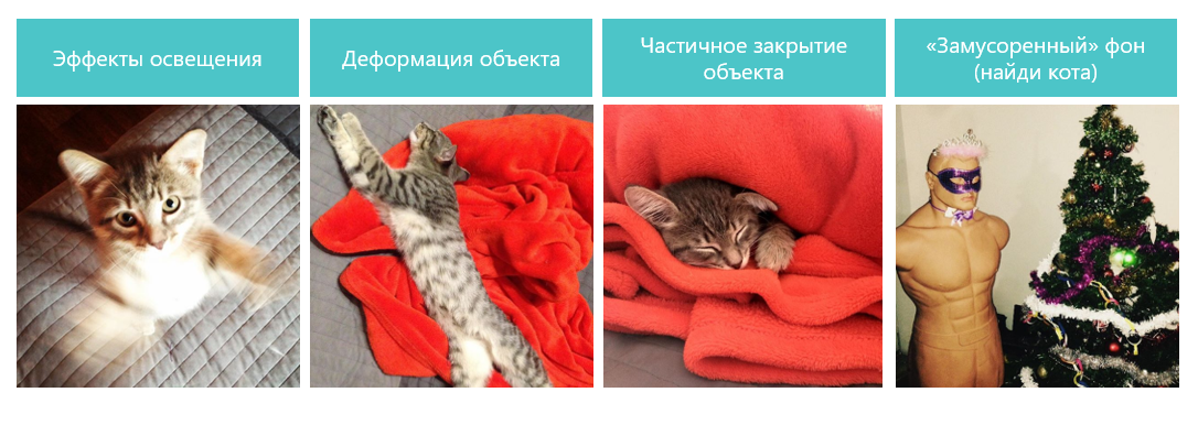
This example in our article is rather “toy”: the authors of the data have already collected them in the hope that they will have to use them for recognition. Accordingly, we chose only good pictures taken under normal lighting not at an angle, etc. Real life is much richer.
We cannot disclose the details of a real project, but here are a number of difficulties that we had to overcome:
- Approximately 150 categories of products that must be found and classified, as well as marked,
- Practically each of these categories has 3-7 styles,
- Often more than 100 products in one shot,
- Sometimes it’s impossible to take a picture of a rack in one photo,
- Poor lighting and backlit vendor play (neon),
- The product behind the glass (glare, the reflection of the photographer),
- Photos from a high angle, when the photographer does not have enough space to take a photo "full face",
- The imposition of goods, as well as situations where the goods stand abutly (SSD can not cope),
- Products on the lower shelves are highly distorted, poorly lit,
- Non-standard shelving.
All this drastically changes and complicates the process of data preparation, training and architecture of used neural networks, but it will not stop us.