Practical bioinformatics, part 4. Getting ready to work with ZINBA
 In the modern world of data analysis, using only one method or only one approach means that sooner or later you will come across the fact how much you were mistaken. Various methods are combined for data analysis, the result is compared, and more accurate forecasts are already made based on the comparison. The ZINBA program uses just such an approach. The developers have combined a variety of methods for analyzing DNA-seq experiments in a single package. This package is written for the statistical data processing program R. What does ZINBA do? It finds various enriched regions even in those cases when some of them were amplified, for example, chemically or have a different degree of signal-to-noise ratio.
 At first, I expected to make a review article about the ZINBA software product ., but the more I read about the methods used in it, the deeper I buried myself in algorithms and definitions. And when in the future he outlined the knowledge gained, he realized the fact that the data had already been collected on more than one article, and without introduction it would be difficult to touch the essence of the issue. In this topic, I give brief excerpts from the articles mentioned in the description of the ZINBA program, supplementing them with my own comments. I will wait for your comments to get to the bottom of the truth together.
Far-reaching plans for regulatory biology are to learn how the genome encodes a variety of mechanisms of gene expression. The relationship between coding and these mechanisms is revealed due to the possibility of finding protein binding sites throughout the genome using chromatin immunoprecipitation ( ChIP) and gene expression (RNA-seq). There is no need to go far for evidence; there is the Encyclopedia of DNA Elements project (ENCODE [1]), within the framework of which most of the functional elements of the genome are recognized. The first steps were taken using the microarray method, but deep DNA sequencing (ChIP-seq & DNA-seq, sometimes the term NGS next generation sequencing is used) caught up with and overtook this technology.
RNA-seq and ChIP-seq have the following positive differences: they increase the accuracy, specificity, measurement sensitivity and allow you to immediately examine the entire genome. In general, RNA-seq and ChIP-seq have some similarities with a predecessor such as a microchip, but the details are very different. But sequencing still suffers from a number of difficulties, although much better than the microchip in these matters. Due to the fact that the cut DNA fragments are rather short, it is likely that the fragments can occur several times in the genome, be parts of the repetitive part of the DNA, or turn out to be common fragments for some start sites.
It is believed that data processing should consider the ChIP reaction as enrichment. Because approximately 60-99% of fragments in the prepared DNA solution are usually the background, and the remaining 1-40% relate to fragments whose protein could cross-link the antibody [2]. It is this smallest part of the solution that will be sequenced. The fact that the level of pollution is high should be taken into account when calculating enrichment. The number of reads per genome in some cases is incomparably small, for example, for the mammalian genome, the number of reads of reads is less than 1% of the total length of the genome. Sequencing data obviously requires new algorithms and software.
 Fig. 1
This slide schematically shows the hierarchy of ChIP-seq and RNA-seq analysis. Typically, the analysis goes through all the steps from the bottom up. Different programs are applied at each level of the circuit and are sometimes divided into programs specifically for ChIP-seq and RNA-seq. The output of one program is the input to another (pipeline). As you can see from the diagram, all programs first go through the definition of reads on the genome (Maps read), with the exception of the assembly of transcripts, the result of which are the alleged transcripts[3]. After the reads are located on the genome, the output of such a program is transferred to the input of the Aggregate and identity program. For example, to determine enriched regions or read density on a known annotation. Also, these programs may include some subsequent analysis of both binding sites (for DNA-seq) and new unexplored fragments of transcription-isoformism (for ChIP-seq). The following is a higher level analysis. It includes the determination of conservative motives or the level of expression, which may result in the discovery of a new gene model. The integration level (Integrate) indicates that for the current data processing, previously obtained results can be used (not necessarily as part of the current experiment, laboratory or country).
So what do we get after the reads were found on the genome? What does this data look like and how do they differ from each other? There are binding sites on the DNA to which one or another protein can attach; we will call these sites binding sites or simply sites. For example, a CTCF site means that the CTCF proteincan gain a foothold in this area. Scientists have found an antibody to the CTCF protein and using the antibody were able to precipitate the corresponding sections of DNA. But, as we already know, along with special sections arbitrary antibodies can attach to the antibody. Other methods work similarly: the protein attaches to DNA, the antibody attaches to the protein, only the sample of DNA regions changes. Thus, the specifics of the selected sections leaves its mark, and the landscape of the drawing for each method will have its own: somewhere narrow peaks, as in the CTCF method, graph a; somewhere steep peaks with a large adjacent territory, for example, RNA polymerase II method, graph b; upon precipitation of the histone modification, a continuous “fringe” is obtained, this is due to the peculiarity of the arrangement of histones, Figure c. On the graphs along the “x” axis, the coordinate on the chromosome is plotted, and along the y axis is the density of the reads. The data for the figure are taken from [4].
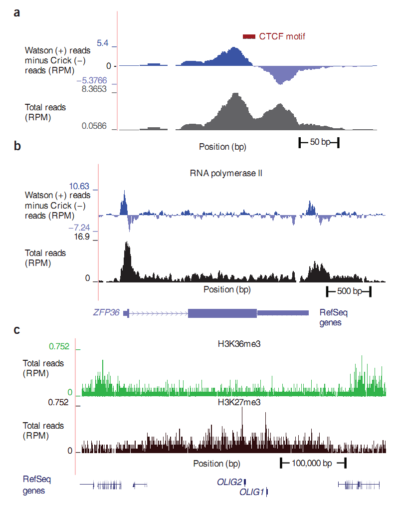 Fig. 2
The presence of the background forces the algorithms to try to evaluate it empirically based on “control”. Control is an additional experiment conducted with the initial solution with special (preimmune) antibodies, with which nothing should connect, but still randomly connects. The result of this connection is some arbitrary background. Some algorithms simulate a possible background, based only on the received data, without control. Whichever approach is chosen (with and without control), the distribution of background reads cannot be completely unified, since the background level depends both on the type of cells and tissue from which they are obtained, and on the deposition method, etc. . Applied technology for amplification (amplification, PCR) and sequencing can also add artificial enrichment (artifacts) or enhance one section more than the other. There are algorithms that allow you to find enriched areas for each experiment. Although each of the algorithms is sharpened for the data corresponding to the experiment, the assumption underlying the algorithm does not always fit the possible set of enriched regions found using DNA-seq [2].
Below, to compare the data, there are graphs from a newer article on ZIMBA. Similar graphs are blurred due to differences in scale between the first and second figures, but they look consistent with the above explanation about DNA-seq technology (see Fig. 2).

Fig. 3
In Fig. 3, in addition to the previous graphs, the landscapes of the following DNA-seq experiments are shown : DNA- sensitive sample (DNase-seq) [5] and protein isolation / fixation using formaldehyde (FAIRE-seq) [6].
DNA is a double helix. This phrase is popular in itself, but it is often forgotten. What does it mean in our case? And the fact that the program that will search for reads on the genome will give out, along with the coordinates on the chromosome, and which side of the spiral (strand) this read is. Spirals are divided into positive (sense) and nonpositive (nonsense / antisense). The mechanism for obtaining reeds is such that most reeds will be located on two different sides relative to the protein associated with DNA. Moreover, in most cases, the reads will be located at the 5 'end of the corresponding spiral. Therefore, the reads on both sides will tend to the center of the protein binding site. Figure 4 shows this schematically, the red dots are the reads from the 5 'end, and in the center is the protein bound to the DNA.
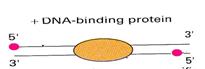
Fig. 4
Thus, to find the center of the protein-DNA binding site, we construct the following graph. To do this, on the “y” axis we postpone the difference between the number of reads from the positive and negative sides, on the “x” axis we postpone the coordinate of the read corresponding to the chromosome. In Figure 5, reads are shown in red on the positive side and blue on the negative side. The resulting graph crosses zero very close to the center of the protein binding site (see bottom graph of Fig. 5). Algorithms exist that, up to the nucleotide, determine binding sites.
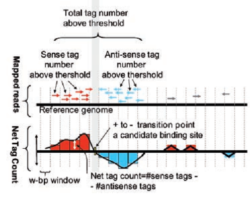
Fig. 5
In this topic, I tried to briefly introduce the material that is the subject of research. Differences in the landscapes of the corresponding DNA-seq experiments were shown, and a method for approximate finding the center of the protein binding site was explained. A huge work lies ahead: we have to understand the differences between the algorithms depending on the landscape, learn how to find peaks and try to distinguish them from artificial ones, find out which regions of the genome lying in the vicinity of the peak can be considered enriched, and all this in order to begin the discussion about the work of ZINBA .
1. Birney, E., et al., Identification and analysis of functional elements in 1% of the human genome by the ENCODE pilot project. Nature, 2007.447 (7146): p. 799-816.
2. Pepke, S., B. Wold, and A. Mortazavi, Computation for ChIP-seq and RNA-seq studies. Nat Methods, 2009.6 (11 Suppl): p. S22-32.
3. Barski, A. and K. Zhao, Genomic location analysis by ChIP-Seq. J Cell Biochem, 2009.107 (1): p. 11-8.
4. Barski, A., et al., High-resolution profiling of histone methylations in the human genome. Cell, 2007.129 (4): p. 823-37.
5. Boyle, AP and TS Furey, High-resolution mapping studies of chromatin and gene regulatory elements. Epigenomics, 2009.1 (2): p. 319-329.
6. Giresi, PG and JD Lieb, Isolation of active regulatory elements from eukaryotic chromatin using FAIRE (Formaldehyde Assisted Isolation of Regulatory Elements). Methods, 2009.48 (3): p. 233-9.
Review is prepared by Andrey Kartashov, Cincinnati, OH, porter@porter.st
corrected by Ekaterina Morozova, ekaterina@porter.st.