Competition Kaggle Home Credit Default Risk - data analysis and simple predictive models
At the datafest 2 in Minsk, Vladimir Iglovikov, a machine vision engineer at Lyft, quite remarkably explained that the best way to learn Data Science is to participate in competitions, run someone else's solutions, combine them, achieve results and show your work. Actually, within the framework of this paradigm, I decided to take a closer look at the Home Credit credit risk assessment competition and explain (to dateologists to beginners and, most of all, to themselves) how to analyze such data correctly and build models for them.

(picture from here )
 Home Credit Group is a group of banks and non-bank credit organizations that operates in 11 countries (including Russia as Home Credit and Finance Bank LLC). The purpose of the competition is to create a methodology for assessing the creditworthiness of borrowers who do not have a credit history. What looks quite noble - borrowers of this category often cannot get any credit from a bank and are forced to turn to scammers and micro-loans. Interestingly, the customer does not expose requirements for transparency and interpretability of the model (as is usually the case in banks), you can use anything, even neural networks.
The training sample consists of 300+ thousand records, there are a lot of signs - 122, among them there are many categorical (not numeric). Signs describe the borrower in some detail, right down to the material from which the walls of his dwelling are made. Part of the data is contained in 6 additional tables (data on the credit bureau, credit card balance and previous loans), these data must also be somehow processed and uploaded to the main one.
Competition looks like a standard classification task (1 in the TARGET field means any difficulties with payments, 0 means no difficulties). However, it is necessary to predict not the 0/1, but the probability of occurrence of problems (which, however, quite easily solve the methods of predicting the predict_proba probabilities that all complex models have).
At first glance, it’s pretty standard for machine learning tasks, the organizers offered a large prize of $ 70k, as a result more than 2600 teams are already participating in the competition, and the battle is taking place for thousandths of a percent. However, on the other hand, such popularity means that dataset has been researched far and wide and created many kernels with good EDA (Exploratory Data Analisys - research and analysis of data in the network, including graphical), Feature engineering'om (working with features) and with interesting models. (Kernel is an example of working with a dataset, which anyone can put in order to show their work to other cagglers.) The
kernels are worth attention:
To work with the data is usually recommended the following plan, which we will try to follow.
In this case, you need to take the amendment to the fact that the data are quite extensive and you can not overpower them right away, it makes sense to act in stages.
Let's start with the import of libraries that we need in the analysis to work with data in the form of tables, graphing and working with matrices.
Load the data. Let's see what we all have. Such an arrangement in the "../input/" directory, by the way, is associated with the requirement for placing its Kernels on Kaggle.
There are 8 data tables (not including the HomeCredit_columns_description.csv table, which contains the description of the fields), which are related as follows:
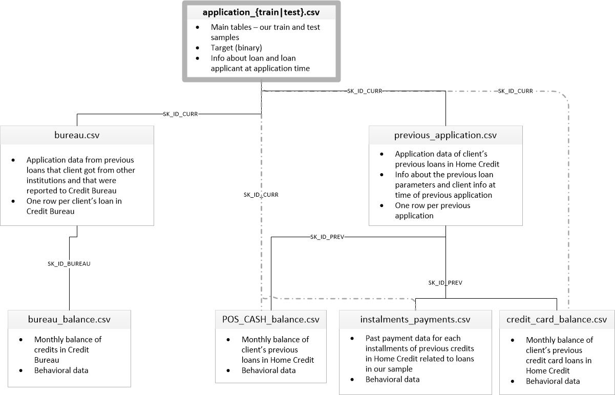
application_train / application_test: Basic data, the borrower is identified by the field SK_ID_CURR
bureau: Data on previous loans in other credit institutions from bureau
bureau_balance: Monthly data on previous bureau loans. Each row - last month it by using a credit
previous_application: Previous applications for loans Home Credit, each has a unique field SK_ID_PREV
POS_CASH_BALANCE: Monthly data on loans to the Home Credits and cash advance loans for the purchase of goods
credit_card_balance: Monthly data on the balance of credit cards in the Home Credit
installments_payment: Billing history of previous loans in Home Credit.
Let's focus for a start on the main data source and see what information can be extracted from it and which models to build. Load the master data.
Total we have 307 thousand records and 122 signs in the training sample and 49 thousand records and 121 signs in the test. The discrepancy is obviously caused by the fact that there is no target TARGET feature in the test sample, which we will predict.
Look at the data carefully
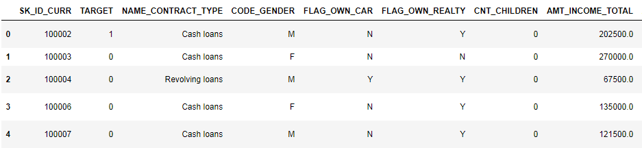
(the first 8 columns are shown)
It is rather difficult to watch data in this format. Let's look at the list of columns: Let me remind you that detailed annotations on the fields are in the file HomeCredit_columns_description. As you can see from info, part of the data is incomplete and part is categorical, they are displayed as object. Most models with such data do not work, we have to do something about it. At this initial analysis can be considered complete, go directly to the EDA
In the EDA process, we consider basic statistics and draw graphs to find trends, anomalies, patterns, and relationships within the data. The purpose of an EDA is to find out what the data can tell. Usually the analysis goes from top to bottom - from a general overview to the study of individual zones that attract attention and may be of interest. Subsequently, these findings can be used in the construction of the model, the choice of features for it and in its interpretation.
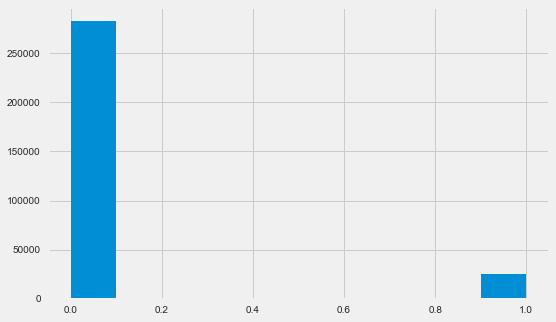
Let me remind you, 1 means problems of any kind with a return, 0 means no problems. As you can see, mostly borrowers have no problems with return, the proportion of problem ones is about 8%. This means that the classes are not balanced and this may need to be taken into account when building the model.
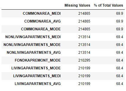
We have seen that the lack of data is quite substantial. Let's see in more detail where and what is missing.
In graphic format:
There are many answers to the question “what to do with all this”. You can fill in with zeros, you can use median values, you can just delete strings without the necessary information. It all depends on the model that we plan to use, as some perfectly cope with the missing values. For now, remember this fact and leave everything as it is.
As we remember. part of the columns is of type object, that is, it has not a numeric value, but reflects some category. Let's look at these columns more closely.
We have 16 columns, in each of which from 2 to 58 different options of values. In general, machine learning models cannot do anything with such columns (except for some, such as LightGBM or CatBoost). Since we plan to try out different models on dataset, we need to do something about it. There are basically two approaches here:
Of the popular ones, the target target encoding is also worth noting (thanks to the roryorangepants for clarifying ).
There is a small problem with Label Encoding - it assigns numeric values that have nothing to do with reality. For example, if we are dealing with a numerical value, then the borrower's income of 100,000 is definitely greater and better than the income of 20,000. But can we say that, for example, one city is better than another because one is assigned the value 100 and the other is 200 ?
One-Hot-encoding, on the other hand, is safer, but can produce “extra” columns. For example, if we encode the same gender with One-Hot, we will have two columns, “male and female”, although one would suffice, “Is it a man?”
According to the good for this dataset, it would be necessary to encode the signs with low variability with the help of Label Encoding, and everything else - One-Hot, but to simplify, we will encode everything using One-Hot. On the speed of calculation and the result is almost no effect. The pandas coding process itself is very simple.
Since the number of options in the sample columns is not equal, the number of columns now does not match. Alignment is required - it is necessary to remove columns that are not in the test one from the training sample. This is done by the align method, you need to specify axis = 1 (for columns).
A good way to understand the data is to calculate the Pearson correlation coefficients for the data relative to the target feature. This is not the best method to show the relevance of the signs, but it is simple and allows you to get an idea of the data. Interpret the coefficients as follows:
Thus, all data weakly correlate with the target (except for the target itself, which, of course, is equal to itself). However, age and some “external data sources” are distinguished from the data. This is probably some additional data from other credit institutions. It's funny that although the goal is declared as independence from such data in making a credit decision, in fact we will be based primarily on them.
It is clear that the older the client, the higher the probability of return (up to a certain limit, of course). But for some reason, the age is specified on negative days before the loan is issued, so it positively correlates with non-return (which looks somewhat strange). Let's bring it to a positive value and look at the correlation.
Let's look at the variable more carefully. Let's start with the histogram.
The distribution histogram itself can say something useful, except that we do not see any particular emissions and everything looks more or less plausible. To show the effect of age on the result, you can construct a graph of kernel density estimation (KDE) - the distribution of nuclear density, painted in the colors of the target feature. It shows the distribution of one variable and can be interpreted as a smoothed histogram (calculated as the Gaussian core over each point, which is then averaged to smooth).
As can be seen, the non-return rate is higher for young people and decreases with increasing age. This is not a reason to always deny young people a loan, such a “recommendation” will only lead to a loss of income and a market for the bank. This is a reason to think about a more thorough tracking of such loans, assessment and, perhaps, even some kind of financial education for young borrowers.
Let's take a closer look at the “external data sources” EXT_SOURCE and their correlation.
It is also convenient to display the correlation using heatmap.
As you can see, all sources show a negative correlation with the target. Let's look at the KDE distribution for each source.
The picture is similar to the distribution by age - with the growth of the indicator, the probability of repayment of a loan increases. The third source is strongest in this regard. Although in absolute terms the correlation with the target variable is still in the “very low” category, external data sources and age will have the highest value in the construction of the model.
For a better understanding of the relationships between these variables, you can build a pair chart, in which we will be able to see the relationships of each pair and the histogram of the distribution diagonally. Above the diagonal, you can show a scatterplot, and below - 2d KDE.
Blue shows returnable loans, red - non-returnable. It is rather difficult to interpret this, but a good print on a T-shirt or a picture can come out of this picture at a museum of modern art.
Let us consider in more detail other signs and their dependence on the target variable. Since there are many categorical ones among them (and we have already managed to encode them), we will need the original data again. Let's call them a little differently to avoid confusion.
We also need a couple of functions to beautifully display the distributions and their effect on the target variable. Many thanks to the author of this kernel here .
So, we will consider the main signs of kolientov
Interestingly, revolving loans (probably overdrafts or something like that) make up less than 10% of the total number of loans. At the same time, the percentage of no return among them is much higher. A good reason to revise the methodology of working with these loans, and maybe even abandon them.
Women clients are almost twice as many men, while men show a much higher risk.
Clients with a machine half as "horseless". The risk on them is almost the same, customers with a machine pay a little better.
Real estate is the opposite picture - customers without it are half as much. The risk for property owners is also slightly less.
While the majority of clients are married, customers in unmarried and single relationships are less risky. Widowers show minimal risk.
Most customers are childless. At the same time, customers with 9 and 11 children show complete non-return.
As the calculation of values shows, these data are statistically insignificant - only 1-2 clients of both categories. However, all three were defaulted, as were half of the clients with 6 children.
The situation is similar - the smaller the mouths, the higher the recurrence.
Single mothers and the unemployed are likely to be cut off at the application stage - there are too few of them in the sample. But consistently show problems.
Here, drivers and security officers are of interest, which are quite numerous and come up with problems more often than other categories.
The higher the education, the better the reflexivity is obvious.
The highest percentage of non-return is observed in Transport: type 3 (16%), Industry: type 13 (13.5%), Industry: type 8 (12.5%) and in Restaurant (up to 12%).
Consider the distribution of loan amounts and their impact on repayment.
As the density plot shows, strong sums come back more often.
Customers from more populated regions tend to pay off loans better.
Thus, we got an idea about the main features of dataset and their influence on the result. Specifically, with the listed in this article we will not do anything, but they can be very important in future work.
Competitions on Kaggle are won by transformation of signs - the one who could create the most useful signs from the data wins. At least for structured data, winning models are now basically different versions of gradient boosting. Most often, it is more efficient to spend time converting features than setting up hyper parameters or selecting models. The model can still be trained only according to the data that are transferred to it. Ensuring that the data is relevant to the task is the primary responsibility of the date of the scientist.
The process of converting attributes can include creating new ones from the available data, choosing the most important ones available, etc. Let's try out this time polynomial signs.
The polynomial method of constructing features consists in the fact that we simply create features that are the degree of the features available and their works. In some cases, such constructed features may have a stronger correlation with the target variable than their “parents”. Although such methods are often used in statistical models, they are much less common in machine learning. However. nothing prevents us from trying them, especially since Scikit-Learn has a class specifically for this purpose - PolynomialFeatures - which creates polynomial features and their products, you only need to specify the source features themselves and the maximum degree to which they need to be built. We use the most powerful effects on the result of 4 signs and degree 3,
Total 35 polynomial and derived attributes. Check their correlation with the target.
So, some signs show a higher correlation than the original ones. It makes sense to try learning with and without them (like so much else in machine learning, this can be determined experimentally). To do this, create a copy of the data frames and add new features there.
In the calculations, it is necessary to make a start from some basic level of the model, below which it is no longer possible to fall. In our case, this could be 0.5 for all test clients - this shows that we absolutely can’t imagine whether the client will return the loan or not. In our case, preliminary work has already been done, and you can use more complex models.
To calculate the logistic regression, we need to take tables with coded categorical features, fill in the missing data and normalize them (lead to values from 0 to 1). All this executes the following code:
We use logistic regression from Scikit-Learn as the first model. Let's take the defol model with one amendment - lower the regularization parameter C to avoid overfitting. The usual syntax is to create a model, train it and predict the probability using predict_proba (we need probability, not 0/1)
Now you can create a file to upload to Kaggle. Create a dataframe from customer IDs and the likelihood of non-return and unload it.
So, the result of our titanic work: 0.673, with the best result today, 0.802.
Logreg does not perform well, try using an improved model - a random forest. This is a much more powerful model that can build hundreds of trees and produce a far more accurate result. Use 100 trees. The scheme of work with the model is the same, completely standard - classifier loading, training. prediction.
the result of a random forest is slightly better - 0.683
Now that we have a model. which does at least something - it's time to test our polynomial signs. Let's do the same with them and compare the result.
the result of a random forest with polynomial signs became worse - 0.633. Which strongly calls into question the need for their use.
Gradient boosting is a “serious model” for machine learning. Practically all last competitions "are dragged" precisely. Let's build a simple model and check its performance.
The result of LightGBM is 0.735, which strongly leaves behind all other models.
The simplest method for interpreting a model is to look at the importance of attributes (which not all models can do). Since our classifier processed the array, it will take some work to re-set the column names in accordance with the columns of this array.
As might be expected, the most important to model all the same 4 features. The importance of attributes is not the best method for interpreting a model, but it allows one to understand the main factors that the model uses for predictions.

Now consider carefully the additional tables and what can be done with them. Immediately begin to prepare the table for further study. But to begin with, we will remove the past voluminous tables from memory, we will clear the memory with the help of the garbage collector and import the necessary libraries for further analysis.
Import the data, immediately remove the target column in a separate column
Immediately encode categorical signs. Earlier we did this, while we coded the training and test samples separately, and then flattened the data. Let's try a slightly different approach - we will find all these categorical signs, combine the data frames, encode them according to the list, and then divide the samples into training and test ones again.

MONTHS_BALANCE - the number of months before the filing date of the loan application. Let's take a closer look at the “statuses”
The statuses mean the following:
C - closed, that is, repaid credit. X - unknown status. 0 - current loan, no delinquency. 1 - 1-30 days overdue, 2 - 31-60 days overdue, and so on up to status 5 - the loan is sold to a third party or written off.
Hence, for example the following characteristics can be distinguished: buro_grouped_size - the number of records in the database buro_grouped_max - maximum balance on the loan buro_grouped_min - the minimum balance on the loan
As well as all of these statuses on the loan can be encoded (using method unstack, and then attach the data to the buro table, the benefit of that SK_ID_BUREAU coincides there and there.

(the first 7 columns are shown)
Quite a lot of data, which, in general, you can try to simply encode with One-Hot-Encoding, group by SK_ID_CURR, average and, thus, prepare for combining with the main table

In the same way, we will encode categorical signs, average them and combine them by current ID.

Encode categorical features and prepare a table for combining

(first 7 columns)
Similar work

(first 7 columns are shown)
Let's create three tables - with average, minimum and maximum values from this table.
And, actually, we will strike on this doubled gradient boosting table!
the result is 0.770.
OK, finally, we’ll try a more complicated procedure with the division into folds, cross-validation and the choice of the best iteration.
Final fast on kaggle 0.783
Definitely continue to work with signs. Investigate the data, select some of the features, combine them, attach additional tables in a different way. You can experiment with hyper parameters of mozheli - there are many directions.
I hope this small compilation has shown you modern methods of data research and the preparation of predictive models. Learn datasens, participate in competitions, be cool!
And once again references to the kernels that helped me prepare this article. The article is also posted in the form of a laptop on the Github , you can download it, dataset and run and experiment.
Will Koehrsen. Start Here: A Gentle Introduction
sban. HomeCreditRisk: Extensive EDA + Baseline [0.772]
Gabriel Preda. Home Credit Default Risk Extensive EDA
Pavan Raj. Loan repayers v / s Loan defaulters - HOME CREDIT
Lem Lordje Ko. 15 lines: Just EXT_SOURCE_x
Shanth. HOME CREDIT - BUREAU DATA - FEATURE ENGINEERING
Dmitriy Kisil. Good_fun_with_LigthGBM
(picture from here )
Home Credit Group is a group of banks and non-bank credit organizations that operates in 11 countries (including Russia as Home Credit and Finance Bank LLC). The purpose of the competition is to create a methodology for assessing the creditworthiness of borrowers who do not have a credit history. What looks quite noble - borrowers of this category often cannot get any credit from a bank and are forced to turn to scammers and micro-loans. Interestingly, the customer does not expose requirements for transparency and interpretability of the model (as is usually the case in banks), you can use anything, even neural networks.The training sample consists of 300+ thousand records, there are a lot of signs - 122, among them there are many categorical (not numeric). Signs describe the borrower in some detail, right down to the material from which the walls of his dwelling are made. Part of the data is contained in 6 additional tables (data on the credit bureau, credit card balance and previous loans), these data must also be somehow processed and uploaded to the main one.
Competition looks like a standard classification task (1 in the TARGET field means any difficulties with payments, 0 means no difficulties). However, it is necessary to predict not the 0/1, but the probability of occurrence of problems (which, however, quite easily solve the methods of predicting the predict_proba probabilities that all complex models have).
At first glance, it’s pretty standard for machine learning tasks, the organizers offered a large prize of $ 70k, as a result more than 2600 teams are already participating in the competition, and the battle is taking place for thousandths of a percent. However, on the other hand, such popularity means that dataset has been researched far and wide and created many kernels with good EDA (Exploratory Data Analisys - research and analysis of data in the network, including graphical), Feature engineering'om (working with features) and with interesting models. (Kernel is an example of working with a dataset, which anyone can put in order to show their work to other cagglers.) The
kernels are worth attention:
- EDA with a detailed description for beginners and simple models
- Deep EDA with Plotly Package + Bureau Data Upload
- Good EDA with Seaborn Package
- Comparative analysis of problem and default borrowers
- 15-line LightGBM on three signs with a final speed of 0.714
- Analysis of signs according to credit bureaus
- Processing add. tables + LightGBM
To work with the data is usually recommended the following plan, which we will try to follow.
- Understanding the problem and familiarization with the data
- Data cleaning and formatting
- EDA
- Base model
- Model improvement
- Interpretation of the model
In this case, you need to take the amendment to the fact that the data are quite extensive and you can not overpower them right away, it makes sense to act in stages.
Let's start with the import of libraries that we need in the analysis to work with data in the form of tables, graphing and working with matrices.
import pandas as pd
import matplotlib.pyplot as plt
import numpy as np
import seaborn as sns
%matplotlib inline
Load the data. Let's see what we all have. Such an arrangement in the "../input/" directory, by the way, is associated with the requirement for placing its Kernels on Kaggle.
import os
PATH="../input/"
print(os.listdir(PATH))
['application_test.csv', 'application_train.csv', 'bureau.csv', 'bureau_balance.csv', 'credit_card_balance.csv', 'HomeCredit_columns_description.csv', 'installments_payments.csv', 'POS_CASH_balance.csv', 'previous_application.csv']There are 8 data tables (not including the HomeCredit_columns_description.csv table, which contains the description of the fields), which are related as follows:
application_train / application_test: Basic data, the borrower is identified by the field SK_ID_CURR
bureau: Data on previous loans in other credit institutions from bureau
bureau_balance: Monthly data on previous bureau loans. Each row - last month it by using a credit
previous_application: Previous applications for loans Home Credit, each has a unique field SK_ID_PREV
POS_CASH_BALANCE: Monthly data on loans to the Home Credits and cash advance loans for the purchase of goods
credit_card_balance: Monthly data on the balance of credit cards in the Home Credit
installments_payment: Billing history of previous loans in Home Credit.
Let's focus for a start on the main data source and see what information can be extracted from it and which models to build. Load the master data.
- app_train = pd.read_csv (PATH + 'application_train.csv',)
- app_test = pd.read_csv (PATH + 'application_test.csv',)
- print ("learning sample format:", app_train.shape)
- print ("test sample format:", app_test.shape)
- format of the training sample: (307511, 122)
- test sample format: (48744, 121)
Total we have 307 thousand records and 122 signs in the training sample and 49 thousand records and 121 signs in the test. The discrepancy is obviously caused by the fact that there is no target TARGET feature in the test sample, which we will predict.
Look at the data carefully
pd.set_option('display.max_columns', None) # иначе pandas не покажет все столбцы
app_train.head()
(the first 8 columns are shown)
It is rather difficult to watch data in this format. Let's look at the list of columns: Let me remind you that detailed annotations on the fields are in the file HomeCredit_columns_description. As you can see from info, part of the data is incomplete and part is categorical, they are displayed as object. Most models with such data do not work, we have to do something about it. At this initial analysis can be considered complete, go directly to the EDA
app_train.info(max_cols=122)

<class 'pandas.core.frame.DataFrame'>

RangeIndex: 307511 entries, 0 to 307510

Data columns (total 122 columns):

SK_ID_CURR 307511 non-null int64

TARGET 307511 non-null int64

NAME_CONTRACT_TYPE 307511 non-null object

CODE_GENDER 307511 non-null object

FLAG_OWN_CAR 307511 non-null object

FLAG_OWN_REALTY 307511 non-null object

CNT_CHILDREN 307511 non-null int64

AMT_INCOME_TOTAL 307511 non-null float64

AMT_CREDIT 307511 non-null float64

AMT_ANNUITY 307499 non-null float64

AMT_GOODS_PRICE 307233 non-null float64

NAME_TYPE_SUITE 306219 non-null object

NAME_INCOME_TYPE 307511 non-null object

NAME_EDUCATION_TYPE 307511 non-null object

NAME_FAMILY_STATUS 307511 non-null object

NAME_HOUSING_TYPE 307511 non-null object

REGION_POPULATION_RELATIVE 307511 non-null float64

DAYS_BIRTH 307511 non-null int64

DAYS_EMPLOYED 307511 non-null int64

DAYS_REGISTRATION 307511 non-null float64

DAYS_ID_PUBLISH 307511 non-null int64

OWN_CAR_AGE 104582 non-null float64

FLAG_MOBIL 307511 non-null int64

FLAG_EMP_PHONE 307511 non-null int64

FLAG_WORK_PHONE 307511 non-null int64

FLAG_CONT_MOBILE 307511 non-null int64

FLAG_PHONE 307511 non-null int64

FLAG_EMAIL 307511 non-null int64

OCCUPATION_TYPE 211120 non-null object

CNT_FAM_MEMBERS 307509 non-null float64

REGION_RATING_CLIENT 307511 non-null int64

REGION_RATING_CLIENT_W_CITY 307511 non-null int64

WEEKDAY_APPR_PROCESS_START 307511 non-null object

HOUR_APPR_PROCESS_START 307511 non-null int64

REG_REGION_NOT_LIVE_REGION 307511 non-null int64

REG_REGION_NOT_WORK_REGION 307511 non-null int64

LIVE_REGION_NOT_WORK_REGION 307511 non-null int64

REG_CITY_NOT_LIVE_CITY 307511 non-null int64

REG_CITY_NOT_WORK_CITY 307511 non-null int64

LIVE_CITY_NOT_WORK_CITY 307511 non-null int64

ORGANIZATION_TYPE 307511 non-null object

EXT_SOURCE_1 134133 non-null float64

EXT_SOURCE_2 306851 non-null float64

EXT_SOURCE_3 246546 non-null float64

APARTMENTS_AVG 151450 non-null float64

BASEMENTAREA_AVG 127568 non-null float64

YEARS_BEGINEXPLUATATION_AVG 157504 non-null float64

YEARS_BUILD_AVG 103023 non-null float64

COMMONAREA_AVG 92646 non-null float64

ELEVATORS_AVG 143620 non-null float64

ENTRANCES_AVG 152683 non-null float64

FLOORSMAX_AVG 154491 non-null float64

FLOORSMIN_AVG 98869 non-null float64

LANDAREA_AVG 124921 non-null float64

LIVINGAPARTMENTS_AVG 97312 non-null float64

LIVINGAREA_AVG 153161 non-null float64

NONLIVINGAPARTMENTS_AVG 93997 non-null float64

NONLIVINGAREA_AVG 137829 non-null float64

APARTMENTS_MODE 151450 non-null float64

BASEMENTAREA_MODE 127568 non-null float64

YEARS_BEGINEXPLUATATION_MODE 157504 non-null float64

YEARS_BUILD_MODE 103023 non-null float64

COMMONAREA_MODE 92646 non-null float64

ELEVATORS_MODE 143620 non-null float64

ENTRANCES_MODE 152683 non-null float64

FLOORSMAX_MODE 154491 non-null float64

FLOORSMIN_MODE 98869 non-null float64

LANDAREA_MODE 124921 non-null float64

LIVINGAPARTMENTS_MODE 97312 non-null float64

LIVINGAREA_MODE 153161 non-null float64

NONLIVINGAPARTMENTS_MODE 93997 non-null float64

NONLIVINGAREA_MODE 137829 non-null float64

APARTMENTS_MEDI 151450 non-null float64

BASEMENTAREA_MEDI 127568 non-null float64

YEARS_BEGINEXPLUATATION_MEDI 157504 non-null float64

YEARS_BUILD_MEDI 103023 non-null float64

COMMONAREA_MEDI 92646 non-null float64

ELEVATORS_MEDI 143620 non-null float64

ENTRANCES_MEDI 152683 non-null float64

FLOORSMAX_MEDI 154491 non-null float64

FLOORSMIN_MEDI 98869 non-null float64

LANDAREA_MEDI 124921 non-null float64

LIVINGAPARTMENTS_MEDI 97312 non-null float64

LIVINGAREA_MEDI 153161 non-null float64

NONLIVINGAPARTMENTS_MEDI 93997 non-null float64

NONLIVINGAREA_MEDI 137829 non-null float64

FONDKAPREMONT_MODE 97216 non-null object

HOUSETYPE_MODE 153214 non-null object

TOTALAREA_MODE 159080 non-null float64

WALLSMATERIAL_MODE 151170 non-null object

EMERGENCYSTATE_MODE 161756 non-null object

OBS_30_CNT_SOCIAL_CIRCLE 306490 non-null float64

DEF_30_CNT_SOCIAL_CIRCLE 306490 non-null float64

OBS_60_CNT_SOCIAL_CIRCLE 306490 non-null float64

DEF_60_CNT_SOCIAL_CIRCLE 306490 non-null float64

DAYS_LAST_PHONE_CHANGE 307510 non-null float64

FLAG_DOCUMENT_2 307511 non-null int64

FLAG_DOCUMENT_3 307511 non-null int64

FLAG_DOCUMENT_4 307511 non-null int64

FLAG_DOCUMENT_5 307511 non-null int64

FLAG_DOCUMENT_6 307511 non-null int64

FLAG_DOCUMENT_7 307511 non-null int64

FLAG_DOCUMENT_8 307511 non-null int64

FLAG_DOCUMENT_9 307511 non-null int64

FLAG_DOCUMENT_10 307511 non-null int64

FLAG_DOCUMENT_11 307511 non-null int64

FLAG_DOCUMENT_12 307511 non-null int64

FLAG_DOCUMENT_13 307511 non-null int64

FLAG_DOCUMENT_14 307511 non-null int64

FLAG_DOCUMENT_15 307511 non-null int64

FLAG_DOCUMENT_16 307511 non-null int64

FLAG_DOCUMENT_17 307511 non-null int64

FLAG_DOCUMENT_18 307511 non-null int64

FLAG_DOCUMENT_19 307511 non-null int64

FLAG_DOCUMENT_20 307511 non-null int64

FLAG_DOCUMENT_21 307511 non-null int64

AMT_REQ_CREDIT_BUREAU_HOUR 265992 non-null float64

AMT_REQ_CREDIT_BUREAU_DAY 265992 non-null float64

AMT_REQ_CREDIT_BUREAU_WEEK 265992 non-null float64

AMT_REQ_CREDIT_BUREAU_MON 265992 non-null float64

AMT_REQ_CREDIT_BUREAU_QRT 265992 non-null float64

AMT_REQ_CREDIT_BUREAU_YEAR 265992 non-null float64

dtypes: float64(65), int64(41), object(16)

memory usage: 286.2+ MB
Exploratory Data Analysis or primary data mining
In the EDA process, we consider basic statistics and draw graphs to find trends, anomalies, patterns, and relationships within the data. The purpose of an EDA is to find out what the data can tell. Usually the analysis goes from top to bottom - from a general overview to the study of individual zones that attract attention and may be of interest. Subsequently, these findings can be used in the construction of the model, the choice of features for it and in its interpretation.
Distribution of target variable
app_train.TARGET.value_counts()0 282686
1 24825
Name: TARGET, dtype: int64plt.style.use('fivethirtyeight')
plt.rcParams["figure.figsize"] = [8,5]
plt.hist(app_train.TARGET)
plt.show()Let me remind you, 1 means problems of any kind with a return, 0 means no problems. As you can see, mostly borrowers have no problems with return, the proportion of problem ones is about 8%. This means that the classes are not balanced and this may need to be taken into account when building the model.
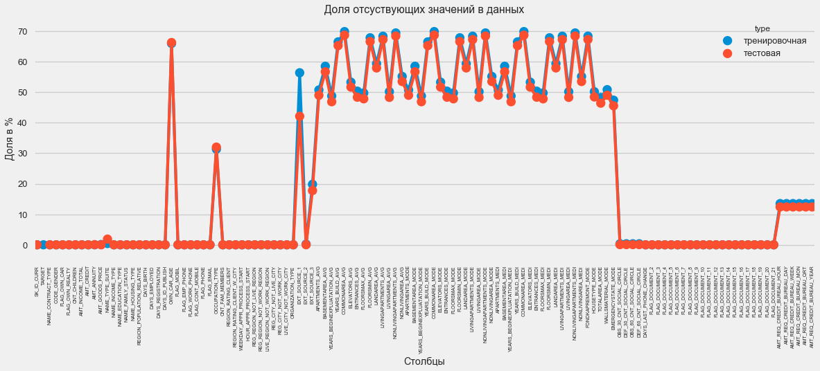
Research missing data
We have seen that the lack of data is quite substantial. Let's see in more detail where and what is missing.
# Функция для подсчета недостающих столбцовdefmissing_values_table(df):# Всего недостает
        mis_val = df.isnull().sum()
        # Процент недостающих данных
        mis_val_percent = 100 * df.isnull().sum() / len(df)
        # Таблица с результатами
        mis_val_table = pd.concat([mis_val, mis_val_percent], axis=1)
        # Переименование столбцов
        mis_val_table_ren_columns = mis_val_table.rename(
        columns = {0 : 'Missing Values', 1 : '% of Total Values'})
        # Сортировка про процентажу
        mis_val_table_ren_columns = mis_val_table_ren_columns[
            mis_val_table_ren_columns.iloc[:,1] != 0].sort_values(
        '% of Total Values', ascending=False).round(1)
        # Инфоprint ("В выбранном датафрейме " + str(df.shape[1]) + " столбцов.\n""Всего " + str(mis_val_table_ren_columns.shape[0]) +
              " столбцов с неполными данными.")
        # Возврат таблицы с даннымиreturn mis_val_table_ren_columns
missing_values = missing_values_table(app_train)
missing_values.head(10)
В выбранном датафрейме 122 столбцов.
Всего 67 столбцов с неполными данными.In graphic format:
plt.style.use('seaborn-talk')
fig = plt.figure(figsize=(18,6))
miss_train = pd.DataFrame((app_train.isnull().sum())*100/app_train.shape[0]).reset_index()
miss_test = pd.DataFrame((app_test.isnull().sum())*100/app_test.shape[0]).reset_index()
miss_train["type"] = "тренировочная"
miss_test["type"] = "тестовая"
missing = pd.concat([miss_train,miss_test],axis=0)
ax = sns.pointplot("index",0,data=missing,hue="type")
plt.xticks(rotation =90,fontsize =7)
plt.title("Доля отсуствующих значений в данных")
plt.ylabel("Доля в %")
plt.xlabel("Столбцы")There are many answers to the question “what to do with all this”. You can fill in with zeros, you can use median values, you can just delete strings without the necessary information. It all depends on the model that we plan to use, as some perfectly cope with the missing values. For now, remember this fact and leave everything as it is.
Types of columns and coding of categorical data
As we remember. part of the columns is of type object, that is, it has not a numeric value, but reflects some category. Let's look at these columns more closely.
app_train.dtypes.value_counts()float64 65
int64 41
object 16
dtype: int64app_train.select_dtypes(include=[object]).apply(pd.Series.nunique, axis = 0)NAME_CONTRACT_TYPE 2
CODE_GENDER 3
FLAG_OWN_CAR 2
FLAG_OWN_REALTY 2
NAME_TYPE_SUITE 7
NAME_INCOME_TYPE 8
NAME_EDUCATION_TYPE 5
NAME_FAMILY_STATUS 6
NAME_HOUSING_TYPE 6
OCCUPATION_TYPE 18
WEEKDAY_APPR_PROCESS_START 7
ORGANIZATION_TYPE 58
FONDKAPREMONT_MODE 4
HOUSETYPE_MODE 3
WALLSMATERIAL_MODE 7
EMERGENCYSTATE_MODE 2
dtype: int64We have 16 columns, in each of which from 2 to 58 different options of values. In general, machine learning models cannot do anything with such columns (except for some, such as LightGBM or CatBoost). Since we plan to try out different models on dataset, we need to do something about it. There are basically two approaches here:
- Label Encoding - categories are assigned numbers 0, 1, 2, and so on, and are written in the same column
- One-Hot-encoding - one column is decomposed into several by the number of variants, and in these columns it is noted which variant of this record.
Of the popular ones, the target target encoding is also worth noting (thanks to the roryorangepants for clarifying ).
There is a small problem with Label Encoding - it assigns numeric values that have nothing to do with reality. For example, if we are dealing with a numerical value, then the borrower's income of 100,000 is definitely greater and better than the income of 20,000. But can we say that, for example, one city is better than another because one is assigned the value 100 and the other is 200 ?
One-Hot-encoding, on the other hand, is safer, but can produce “extra” columns. For example, if we encode the same gender with One-Hot, we will have two columns, “male and female”, although one would suffice, “Is it a man?”
According to the good for this dataset, it would be necessary to encode the signs with low variability with the help of Label Encoding, and everything else - One-Hot, but to simplify, we will encode everything using One-Hot. On the speed of calculation and the result is almost no effect. The pandas coding process itself is very simple.
app_train = pd.get_dummies(app_train)
app_test = pd.get_dummies(app_test)
print('Training Features shape: ', app_train.shape)
print('Testing Features shape: ', app_test.shape)Training Features shape: (307511, 246)
Testing Features shape: (48744, 242)Since the number of options in the sample columns is not equal, the number of columns now does not match. Alignment is required - it is necessary to remove columns that are not in the test one from the training sample. This is done by the align method, you need to specify axis = 1 (for columns).
#сохраним лейблы, их же нет в тестовой выборке и при выравнивании они потеряются.
train_labels = app_train['TARGET']
# Выравнивание - сохранятся только столбцы. имеющиеся в обоих датафреймах
app_train, app_test = app_train.align(app_test, join = 'inner', axis = 1)
print('Формат тренировочной выборки: ', app_train.shape)
print('Формат тестовой выборки: ', app_test.shape)
# Add target back in to the data
app_train['TARGET'] = train_labelsФормат тренировочной выборки: (307511, 242)
Формат тестовой выборки: (48744, 242)Data correlation
A good way to understand the data is to calculate the Pearson correlation coefficients for the data relative to the target feature. This is not the best method to show the relevance of the signs, but it is simple and allows you to get an idea of the data. Interpret the coefficients as follows:
- 00-.19 “very weak”
- 20-.39 “weak”
- 40-.59 “average”
- 60-.79 “strong”
- 80-1.0 “very strong”
# Корреляция и сортировка
correlations = app_train.corr()['TARGET'].sort_values()
# Отображение
print('Наивысшая позитивная корреляция: \n', correlations.tail(15))
print('\nНаивысшая негативная корреляция: \n', correlations.head(15))Наивысшая позитивная корреляция:
DAYS_REGISTRATION 0.041975
OCCUPATION_TYPE_Laborers 0.043019
FLAG_DOCUMENT_3 0.044346
REG_CITY_NOT_LIVE_CITY 0.044395
FLAG_EMP_PHONE 0.045982
NAME_EDUCATION_TYPE_Secondary / secondary special 0.049824
REG_CITY_NOT_WORK_CITY 0.050994
DAYS_ID_PUBLISH 0.051457
CODE_GENDER_M 0.054713
DAYS_LAST_PHONE_CHANGE 0.055218
NAME_INCOME_TYPE_Working 0.057481
REGION_RATING_CLIENT 0.058899
REGION_RATING_CLIENT_W_CITY 0.060893
DAYS_BIRTH 0.078239
TARGET 1.000000
Name: TARGET, dtype: float64
Наивысшая негативная корреляция:
EXT_SOURCE_3 -0.178919
EXT_SOURCE_2 -0.160472
EXT_SOURCE_1 -0.155317
NAME_EDUCATION_TYPE_Higher education -0.056593
CODE_GENDER_F -0.054704
NAME_INCOME_TYPE_Pensioner -0.046209
ORGANIZATION_TYPE_XNA -0.045987
DAYS_EMPLOYED -0.044932
FLOORSMAX_AVG -0.044003
FLOORSMAX_MEDI -0.043768
FLOORSMAX_MODE -0.043226
EMERGENCYSTATE_MODE_No -0.042201
HOUSETYPE_MODE_block of flats -0.040594
AMT_GOODS_PRICE -0.039645
REGION_POPULATION_RELATIVE -0.037227
Name: TARGET, dtype: float64Thus, all data weakly correlate with the target (except for the target itself, which, of course, is equal to itself). However, age and some “external data sources” are distinguished from the data. This is probably some additional data from other credit institutions. It's funny that although the goal is declared as independence from such data in making a credit decision, in fact we will be based primarily on them.
Age
It is clear that the older the client, the higher the probability of return (up to a certain limit, of course). But for some reason, the age is specified on negative days before the loan is issued, so it positively correlates with non-return (which looks somewhat strange). Let's bring it to a positive value and look at the correlation.
app_train['DAYS_BIRTH'] = abs(app_train['DAYS_BIRTH'])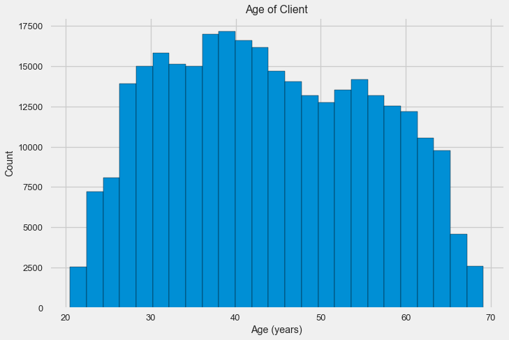
app_train['DAYS_BIRTH'].corr(app_train['TARGET'])-0.078239308309827088Let's look at the variable more carefully. Let's start with the histogram.
# Гистограмма распределения возраста в годах, всего 25 столбцов
plt.hist(app_train['DAYS_BIRTH'] / 365, edgecolor = 'k', bins = 25)
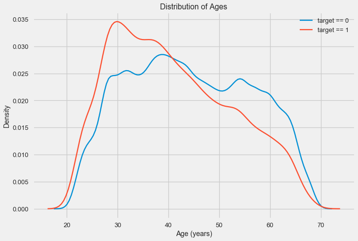
plt.title('Age of Client'); plt.xlabel('Age (years)'); plt.ylabel('Count');The distribution histogram itself can say something useful, except that we do not see any particular emissions and everything looks more or less plausible. To show the effect of age on the result, you can construct a graph of kernel density estimation (KDE) - the distribution of nuclear density, painted in the colors of the target feature. It shows the distribution of one variable and can be interpreted as a smoothed histogram (calculated as the Gaussian core over each point, which is then averaged to smooth).
# KDE займов, выплаченных вовремя
sns.kdeplot(app_train.loc[app_train['TARGET'] == 0, 'DAYS_BIRTH'] / 365, label = 'target == 0')
# KDE проблемных займов
sns.kdeplot(app_train.loc[app_train['TARGET'] == 1, 'DAYS_BIRTH'] / 365, label = 'target == 1')
# Обозначения
plt.xlabel('Age (years)'); plt.ylabel('Density'); plt.title('Distribution of Ages');As can be seen, the non-return rate is higher for young people and decreases with increasing age. This is not a reason to always deny young people a loan, such a “recommendation” will only lead to a loss of income and a market for the bank. This is a reason to think about a more thorough tracking of such loans, assessment and, perhaps, even some kind of financial education for young borrowers.
External sources
Let's take a closer look at the “external data sources” EXT_SOURCE and their correlation.
ext_data = app_train[['TARGET', 'EXT_SOURCE_1', 'EXT_SOURCE_2', 'EXT_SOURCE_3', 'DAYS_BIRTH']]
ext_data_corrs = ext_data.corr()
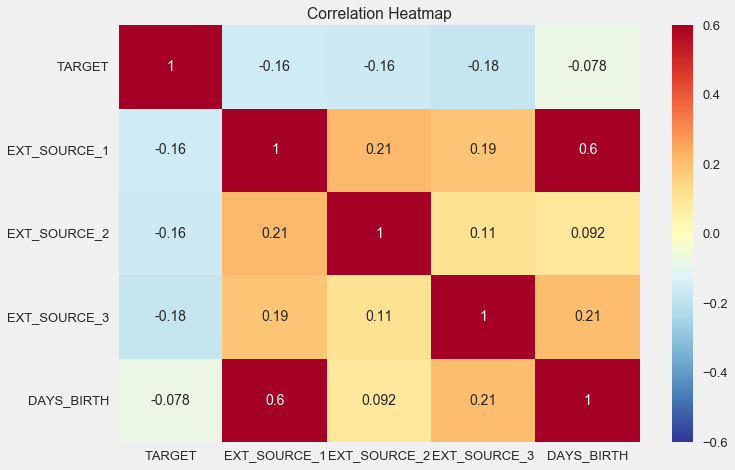
ext_data_corrsIt is also convenient to display the correlation using heatmap.
sns.heatmap(ext_data_corrs, cmap = plt.cm.RdYlBu_r, vmin = -0.25, annot = True, vmax = 0.6)
plt.title('Correlation Heatmap');
As you can see, all sources show a negative correlation with the target. Let's look at the KDE distribution for each source.
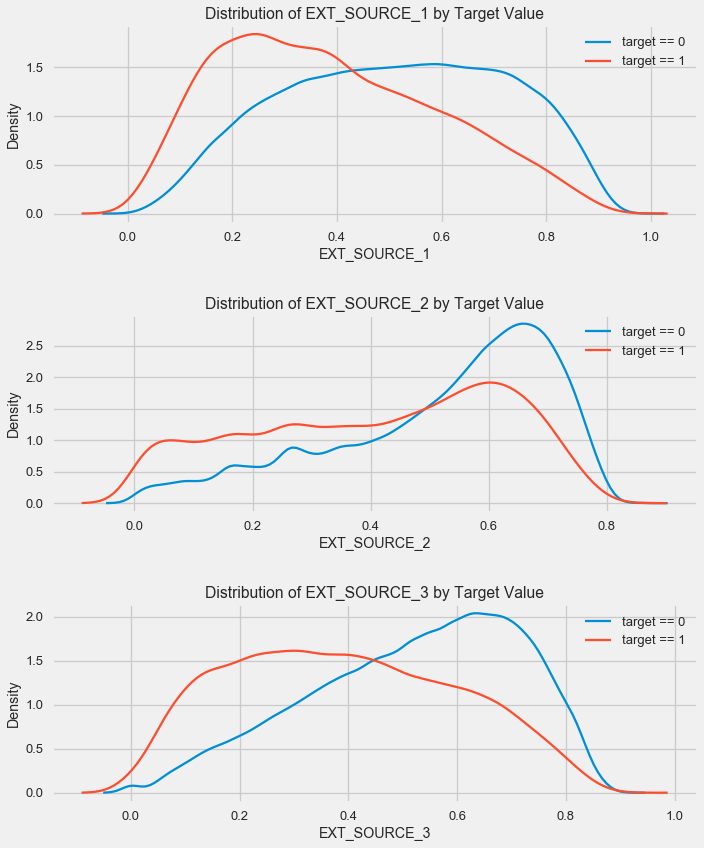
plt.figure(figsize = (10, 12))
# итерация по источникамfor i, source in enumerate(['EXT_SOURCE_1', 'EXT_SOURCE_2', 'EXT_SOURCE_3']):
# сабплот
plt.subplot(3, 1, i + 1)
# отрисовка качественных займов
sns.kdeplot(app_train.loc[app_train['TARGET'] == 0, source], label = 'target == 0')
# отрисовка дефолтных займов
sns.kdeplot(app_train.loc[app_train['TARGET'] == 1, source], label = 'target == 1')
# метки
plt.title('Distribution of %s by Target Value' % source)
plt.xlabel('%s' % source); plt.ylabel('Density');
plt.tight_layout(h_pad = 2.5)The picture is similar to the distribution by age - with the growth of the indicator, the probability of repayment of a loan increases. The third source is strongest in this regard. Although in absolute terms the correlation with the target variable is still in the “very low” category, external data sources and age will have the highest value in the construction of the model.
Pair schedule
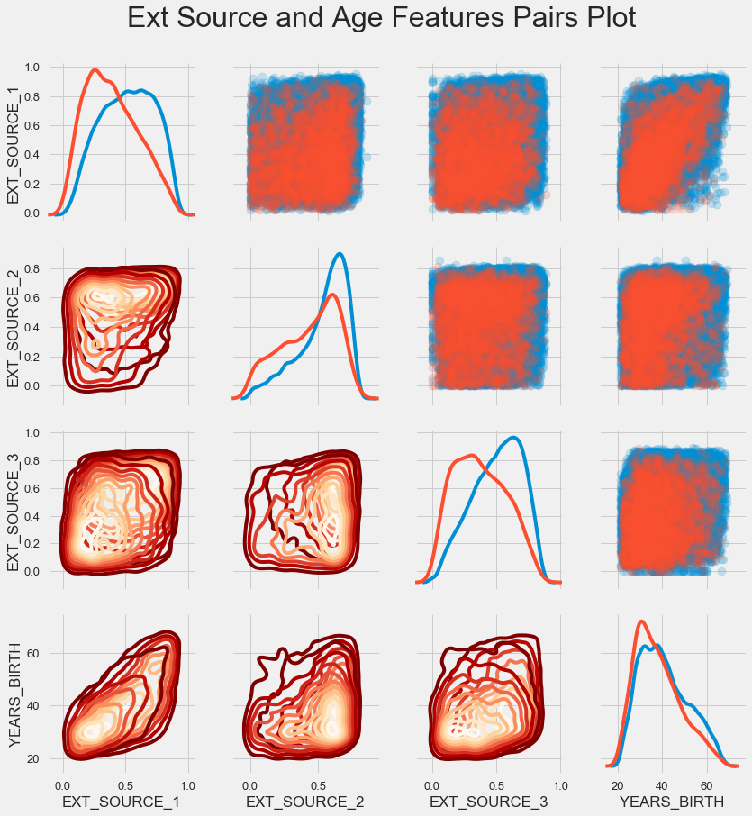
For a better understanding of the relationships between these variables, you can build a pair chart, in which we will be able to see the relationships of each pair and the histogram of the distribution diagonally. Above the diagonal, you can show a scatterplot, and below - 2d KDE.
#вынесем данные по возрасту в отдельный датафрейм
age_data = app_train[['TARGET', 'DAYS_BIRTH']]
age_data['YEARS_BIRTH'] = age_data['DAYS_BIRTH'] / 365
# копирование данных для графика
plot_data = ext_data.drop(labels = ['DAYS_BIRTH'], axis=1).copy()
# Добавим возраст
plot_data['YEARS_BIRTH'] = age_data['YEARS_BIRTH']
# Уберем все незаполненнные строки и ограничим таблицу в 100 тыс. строк
plot_data = plot_data.dropna().loc[:100000, :]
# Функиця для расчет корреляцииdefcorr_func(x, y, **kwargs):
r = np.corrcoef(x, y)[0][1]
ax = plt.gca()
ax.annotate("r = {:.2f}".format(r),
xy=(.2, .8), xycoords=ax.transAxes,
size = 20)
# Создание объекта pairgrid object
grid = sns.PairGrid(data = plot_data, size = 3, diag_sharey=False,
hue = 'TARGET',
vars = [x for x in list(plot_data.columns) if x != 'TARGET'])
# Сверху - скаттерплот
grid.map_upper(plt.scatter, alpha = 0.2)
# Диагональ - гистограмма
grid.map_diag(sns.kdeplot)
# Внизу - распределение плотности
grid.map_lower(sns.kdeplot, cmap = plt.cm.OrRd_r);
plt.suptitle('Ext Source and Age Features Pairs Plot', size = 32, y = 1.05);Blue shows returnable loans, red - non-returnable. It is rather difficult to interpret this, but a good print on a T-shirt or a picture can come out of this picture at a museum of modern art.
Research other signs
Let us consider in more detail other signs and their dependence on the target variable. Since there are many categorical ones among them (and we have already managed to encode them), we will need the original data again. Let's call them a little differently to avoid confusion.
application_train = pd.read_csv(PATH+"application_train.csv")
application_test = pd.read_csv(PATH+"application_test.csv")
We also need a couple of functions to beautifully display the distributions and their effect on the target variable. Many thanks to the author of this kernel here .
defplot_stats(feature,label_rotation=False,horizontal_layout=True):
temp = application_train[feature].value_counts()
df1 = pd.DataFrame({feature: temp.index,'Количество займов': temp.values})
# Расчет доли target=1 в категории
cat_perc = application_train[[feature, 'TARGET']].groupby([feature],as_index=False).mean()
cat_perc.sort_values(by='TARGET', ascending=False, inplace=True)
if(horizontal_layout):
fig, (ax1, ax2) = plt.subplots(ncols=2, figsize=(12,6))
else:
fig, (ax1, ax2) = plt.subplots(nrows=2, figsize=(12,14))
sns.set_color_codes("pastel")
s = sns.barplot(ax=ax1, x = feature, y="Количество займов",data=df1)
if(label_rotation):
s.set_xticklabels(s.get_xticklabels(),rotation=90)
s = sns.barplot(ax=ax2, x = feature, y='TARGET', order=cat_perc[feature], data=cat_perc)
if(label_rotation):
s.set_xticklabels(s.get_xticklabels(),rotation=90)
plt.ylabel('Доля проблемных', fontsize=10)
plt.tick_params(axis='both', which='major', labelsize=10)
plt.show();So, we will consider the main signs of kolientov
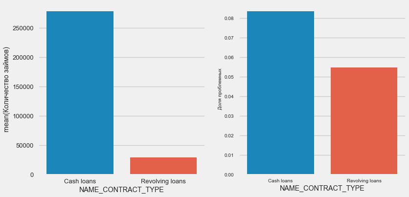
Type of loan
plot_stats('NAME_CONTRACT_TYPE')Interestingly, revolving loans (probably overdrafts or something like that) make up less than 10% of the total number of loans. At the same time, the percentage of no return among them is much higher. A good reason to revise the methodology of working with these loans, and maybe even abandon them.
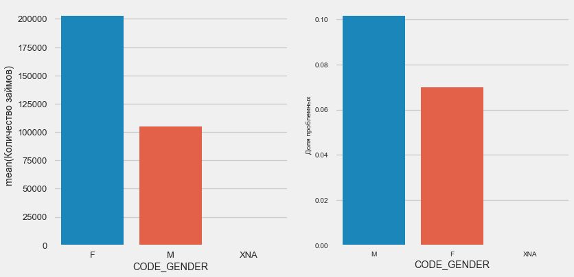
Customer gender
plot_stats('CODE_GENDER')Women clients are almost twice as many men, while men show a much higher risk.
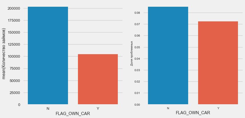
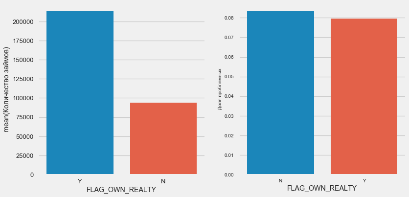
Owning a car and real estate
plot_stats('FLAG_OWN_CAR')
plot_stats('FLAG_OWN_REALTY')
Clients with a machine half as "horseless". The risk on them is almost the same, customers with a machine pay a little better.
Real estate is the opposite picture - customers without it are half as much. The risk for property owners is also slightly less.
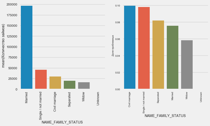
Family status
plot_stats('NAME_FAMILY_STATUS',True, True)While the majority of clients are married, customers in unmarried and single relationships are less risky. Widowers show minimal risk.
Amount of children
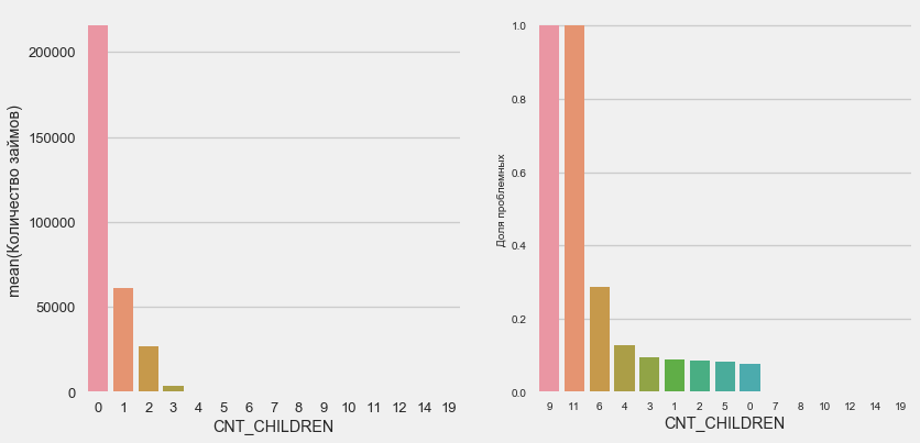
plot_stats('CNT_CHILDREN')Most customers are childless. At the same time, customers with 9 and 11 children show complete non-return.
application_train.CNT_CHILDREN.value_counts()0 215371
1 61119
2 26749
3 3717
4 429
5 84
6 21
7 7
14 3
19 2
12 2
10 2
9 2
8 2
11 1
Name: CNT_CHILDREN, dtype: int64As the calculation of values shows, these data are statistically insignificant - only 1-2 clients of both categories. However, all three were defaulted, as were half of the clients with 6 children.
Number of family members
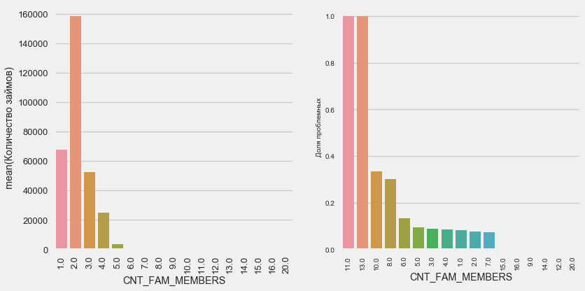
plot_stats('CNT_FAM_MEMBERS',True)The situation is similar - the smaller the mouths, the higher the recurrence.
Type of income
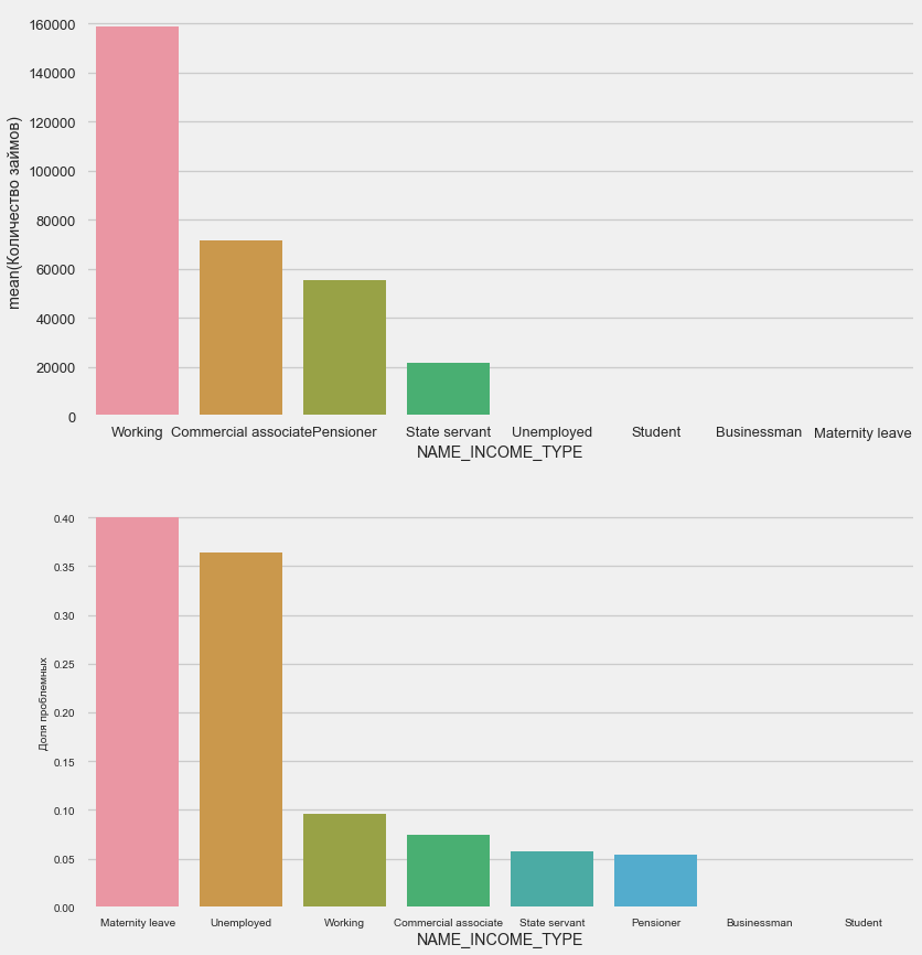
plot_stats('NAME_INCOME_TYPE',False,False)Single mothers and the unemployed are likely to be cut off at the application stage - there are too few of them in the sample. But consistently show problems.
Kind of activity
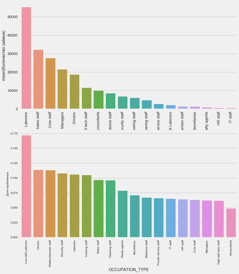
plot_stats('OCCUPATION_TYPE',True, False)application_train.OCCUPATION_TYPE.value_counts()Laborers 55186
Sales staff 32102
Core staff 27570
Managers 21371
Drivers 18603
High skill tech staff 11380
Accountants 9813
Medicine staff 8537
Security staff 6721
Cooking staff 5946
Cleaning staff 4653
Private service staff 2652
Low-skill Laborers 2093
Waiters/barmen staff 1348
Secretaries 1305
Realty agents 751
HR staff 563
IT staff 526
Name: OCCUPATION_TYPE, dtype: int64Here, drivers and security officers are of interest, which are quite numerous and come up with problems more often than other categories.
Education
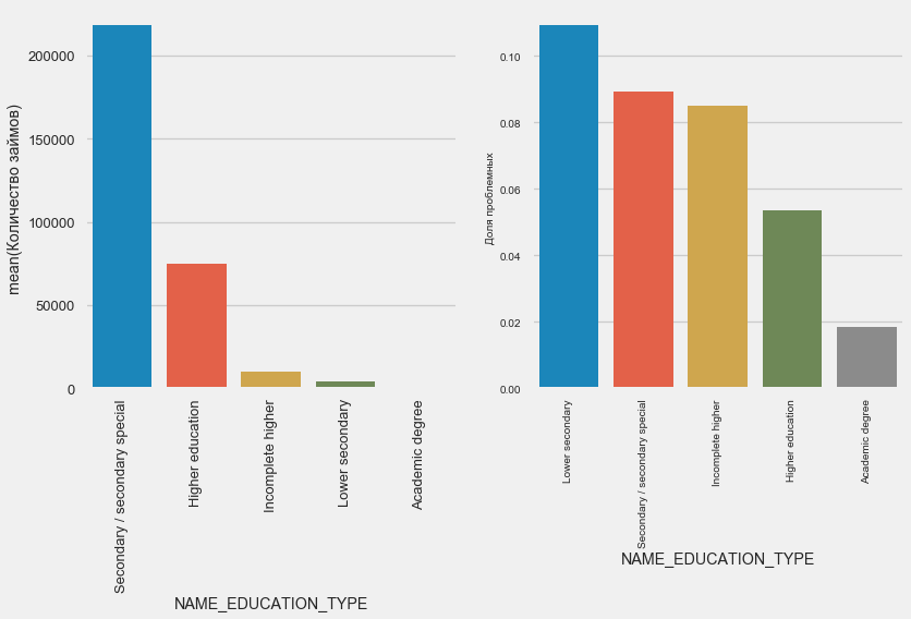
plot_stats('NAME_EDUCATION_TYPE',True)The higher the education, the better the reflexivity is obvious.
Type of organization - employer
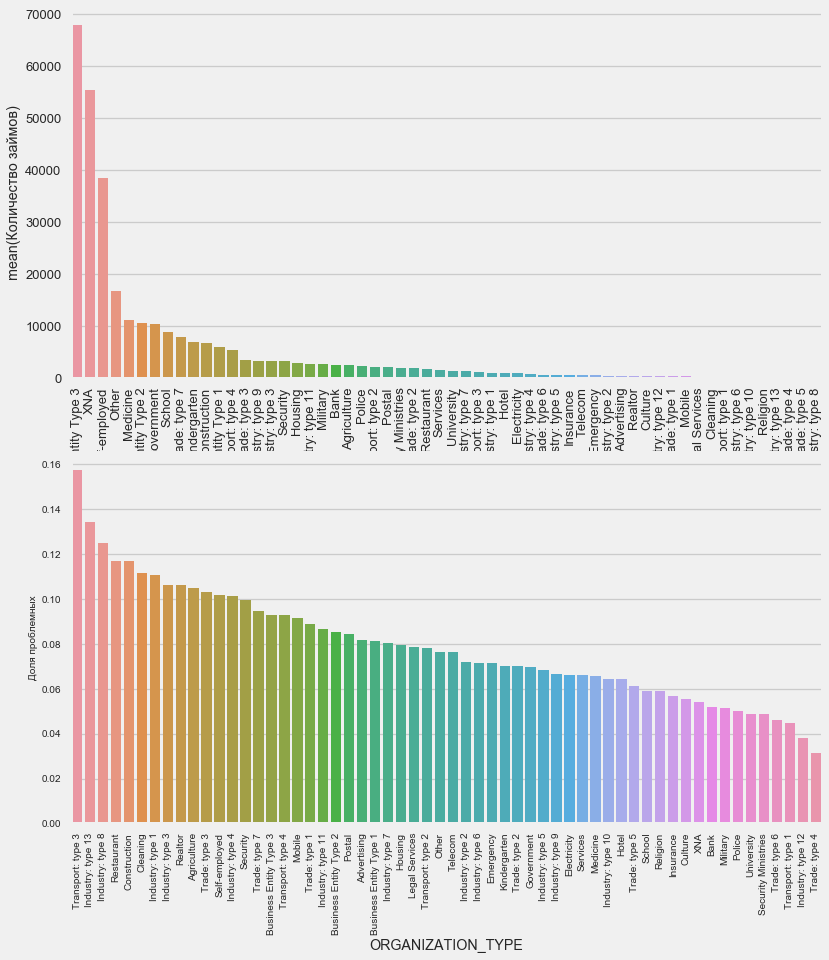
plot_stats('ORGANIZATION_TYPE',True, False)The highest percentage of non-return is observed in Transport: type 3 (16%), Industry: type 13 (13.5%), Industry: type 8 (12.5%) and in Restaurant (up to 12%).
Loan Amount Distribution
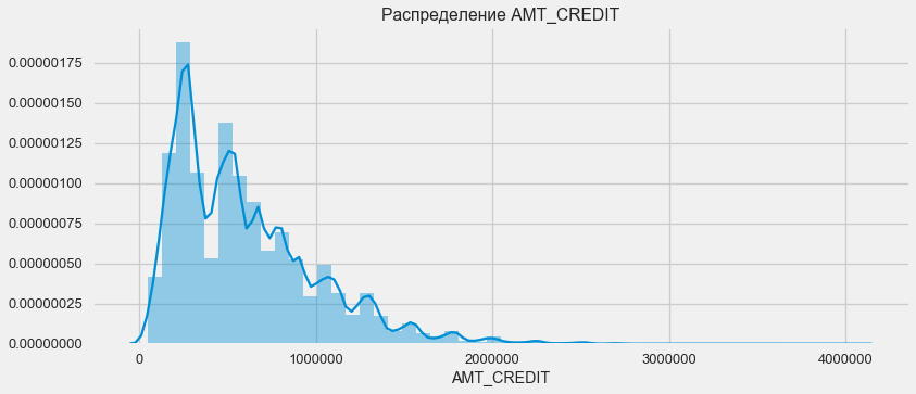
Consider the distribution of loan amounts and their impact on repayment.
plt.figure(figsize=(12,5))
plt.title("Распределение AMT_CREDIT")
ax = sns.distplot(app_train["AMT_CREDIT"])plt.figure(figsize=(12,5))
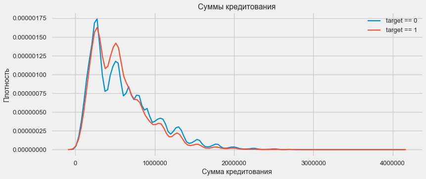
# KDE займов, выплаченных вовремя
sns.kdeplot(app_train.loc[app_train['TARGET'] == 0, 'AMT_CREDIT'], label = 'target == 0')
# KDE проблемных займов
sns.kdeplot(app_train.loc[app_train['TARGET'] == 1, 'AMT_CREDIT'], label = 'target == 1')
# Обозначения
plt.xlabel('Сумма кредитования'); plt.ylabel('Плотность'); plt.title('Суммы кредитования');As the density plot shows, strong sums come back more often.
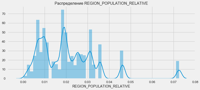
Density distribution
plt.figure(figsize=(12,5))
plt.title("Распределение REGION_POPULATION_RELATIVE")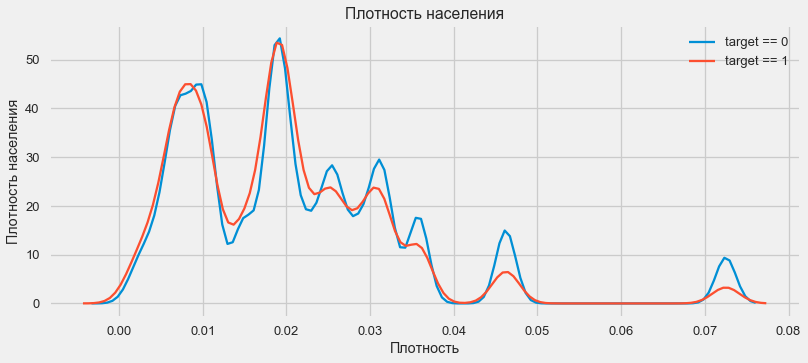
ax = sns.distplot(app_train["REGION_POPULATION_RELATIVE"])plt.figure(figsize=(12,5))
# KDE займов, выплаченных вовремя
sns.kdeplot(app_train.loc[app_train['TARGET'] == 0, 'REGION_POPULATION_RELATIVE'], label = 'target == 0')
# KDE проблемных займов
sns.kdeplot(app_train.loc[app_train['TARGET'] == 1, 'REGION_POPULATION_RELATIVE'], label = 'target == 1')
# Обозначения
plt.xlabel('Плотность'); plt.ylabel('Плотность населения'); plt.title('Плотность населения');Customers from more populated regions tend to pay off loans better.
Thus, we got an idea about the main features of dataset and their influence on the result. Specifically, with the listed in this article we will not do anything, but they can be very important in future work.
Feature Engineering - feature conversion
Competitions on Kaggle are won by transformation of signs - the one who could create the most useful signs from the data wins. At least for structured data, winning models are now basically different versions of gradient boosting. Most often, it is more efficient to spend time converting features than setting up hyper parameters or selecting models. The model can still be trained only according to the data that are transferred to it. Ensuring that the data is relevant to the task is the primary responsibility of the date of the scientist.
The process of converting attributes can include creating new ones from the available data, choosing the most important ones available, etc. Let's try out this time polynomial signs.
Polynomial features
The polynomial method of constructing features consists in the fact that we simply create features that are the degree of the features available and their works. In some cases, such constructed features may have a stronger correlation with the target variable than their “parents”. Although such methods are often used in statistical models, they are much less common in machine learning. However. nothing prevents us from trying them, especially since Scikit-Learn has a class specifically for this purpose - PolynomialFeatures - which creates polynomial features and their products, you only need to specify the source features themselves and the maximum degree to which they need to be built. We use the most powerful effects on the result of 4 signs and degree 3,
# создадим новый датафрейм для полиномиальных признаков
poly_features = app_train[['EXT_SOURCE_1', 'EXT_SOURCE_2', 'EXT_SOURCE_3', 'DAYS_BIRTH', 'TARGET']]
poly_features_test = app_test[['EXT_SOURCE_1', 'EXT_SOURCE_2', 'EXT_SOURCE_3', 'DAYS_BIRTH']]
# обработаем отуствующие данныеfrom sklearn.preprocessing import Imputer
imputer = Imputer(strategy = 'median')
poly_target = poly_features['TARGET']
poly_features = poly_features.drop('TARGET', axis=1)
poly_features = imputer.fit_transform(poly_features)
poly_features_test = imputer.transform(poly_features_test)
from sklearn.preprocessing import PolynomialFeatures
# Создадим полиномиальный объект степени 3
poly_transformer = PolynomialFeatures(degree = 3)
# Тренировка полиномиальных признаков
poly_transformer.fit(poly_features)
# Трансформация признаков
poly_features = poly_transformer.transform(poly_features)
poly_features_test = poly_transformer.transform(poly_features_test)
print('Формат полиномиальных признаков: ', poly_features.shape)Формат полиномиальных признаков: (307511, 35)
Присвоить признакам имена можно при помощи метода get_feature_namespoly_transformer.get_feature_names(input_features = ['EXT_SOURCE_1', 'EXT_SOURCE_2', 'EXT_SOURCE_3', 'DAYS_BIRTH'])[:15]['1',
'EXT_SOURCE_1',
'EXT_SOURCE_2',
'EXT_SOURCE_3',
'DAYS_BIRTH',
'EXT_SOURCE_1^2',
'EXT_SOURCE_1 EXT_SOURCE_2',
'EXT_SOURCE_1 EXT_SOURCE_3',
'EXT_SOURCE_1 DAYS_BIRTH',
'EXT_SOURCE_2^2',
'EXT_SOURCE_2 EXT_SOURCE_3',
'EXT_SOURCE_2 DAYS_BIRTH',
'EXT_SOURCE_3^2',
'EXT_SOURCE_3 DAYS_BIRTH',
'DAYS_BIRTH^2']Total 35 polynomial and derived attributes. Check their correlation with the target.
# Датафрейм для новых фич
poly_features = pd.DataFrame(poly_features,
columns = poly_transformer.get_feature_names(['EXT_SOURCE_1', 'EXT_SOURCE_2',
'EXT_SOURCE_3', 'DAYS_BIRTH']))
# Добавим таргет
poly_features['TARGET'] = poly_target
# рассчитаем корреляцию
poly_corrs = poly_features.corr()['TARGET'].sort_values()
# Отобразим признаки с наивысшей корреляцией
print(poly_corrs.head(10))
print(poly_corrs.tail(5))EXT_SOURCE_2 EXT_SOURCE_3 -0.193939
EXT_SOURCE_1 EXT_SOURCE_2 EXT_SOURCE_3 -0.189605
EXT_SOURCE_2 EXT_SOURCE_3 DAYS_BIRTH -0.181283
EXT_SOURCE_2^2 EXT_SOURCE_3 -0.176428
EXT_SOURCE_2 EXT_SOURCE_3^2 -0.172282
EXT_SOURCE_1 EXT_SOURCE_2 -0.166625
EXT_SOURCE_1 EXT_SOURCE_3 -0.164065
EXT_SOURCE_2 -0.160295
EXT_SOURCE_2 DAYS_BIRTH -0.156873
EXT_SOURCE_1 EXT_SOURCE_2^2 -0.156867
Name: TARGET, dtype: float64
DAYS_BIRTH -0.078239
DAYS_BIRTH^2 -0.076672
DAYS_BIRTH^3 -0.074273
TARGET 1.000000
1 NaN
Name: TARGET, dtype: float64So, some signs show a higher correlation than the original ones. It makes sense to try learning with and without them (like so much else in machine learning, this can be determined experimentally). To do this, create a copy of the data frames and add new features there.
# загрузим тестовые признаки в датафрейм
poly_features_test = pd.DataFrame(poly_features_test,
columns = poly_transformer.get_feature_names(['EXT_SOURCE_1', 'EXT_SOURCE_2',
'EXT_SOURCE_3', 'DAYS_BIRTH']))
# объединим тренировочные датафреймы
poly_features['SK_ID_CURR'] = app_train['SK_ID_CURR']
app_train_poly = app_train.merge(poly_features, on = 'SK_ID_CURR', how = 'left')
# объединим тестовые датафреймы
poly_features_test['SK_ID_CURR'] = app_test['SK_ID_CURR']
app_test_poly = app_test.merge(poly_features_test, on = 'SK_ID_CURR', how = 'left')
# Выровняем датафреймы
app_train_poly, app_test_poly = app_train_poly.align(app_test_poly, join = 'inner', axis = 1)
# Посмотрим формат
print('Тренировочная выборка с полиномиальными признаками: ', app_train_poly.shape)
print('Тестовая выборка с полиномиальными признаками: ', app_test_poly.shape)Тренировочная выборка с полиномиальными признаками: (307511, 277)
Тестовая выборка с полиномиальными признаками: (48744, 277)Model training
A basic level of
In the calculations, it is necessary to make a start from some basic level of the model, below which it is no longer possible to fall. In our case, this could be 0.5 for all test clients - this shows that we absolutely can’t imagine whether the client will return the loan or not. In our case, preliminary work has already been done, and you can use more complex models.
Logistic regression
To calculate the logistic regression, we need to take tables with coded categorical features, fill in the missing data and normalize them (lead to values from 0 to 1). All this executes the following code:
from sklearn.preprocessing import MinMaxScaler, Imputer
# Уберем таргет из тренировочных данныхif'TARGET'in app_train:
train = app_train.drop(labels = ['TARGET'], axis=1)
else:
train = app_train.copy()
features = list(train.columns)
# копируем тестовые данные
test = app_test.copy()
# заполним недостающее по медиане
imputer = Imputer(strategy = 'median')
# Нормализация
scaler = MinMaxScaler(feature_range = (0, 1))
# заполнение тренировочной выборки
imputer.fit(train)
# Трансофрмация тренировочной и тестовой выборок
train = imputer.transform(train)
test = imputer.transform(app_test)
# то же самое с нормализацией
scaler.fit(train)
train = scaler.transform(train)
test = scaler.transform(test)
print('Формат тренировочной выборки: ', train.shape)
print('Формат тестовой выборки: ', test.shape)Формат тренировочной выборки: (307511, 242)
Формат тестовой выборки: (48744, 242)We use logistic regression from Scikit-Learn as the first model. Let's take the defol model with one amendment - lower the regularization parameter C to avoid overfitting. The usual syntax is to create a model, train it and predict the probability using predict_proba (we need probability, not 0/1)
from sklearn.linear_model import LogisticRegression
# Создаем модель
log_reg = LogisticRegression(C = 0.0001)
# Тренируем модель
log_reg.fit(train, train_labels)
LogisticRegression(C=0.0001, class_weight=None, dual=False,
fit_intercept=True, intercept_scaling=1, max_iter=100,
multi_class='ovr', n_jobs=1, penalty='l2', random_state=None,
solver='liblinear', tol=0.0001, verbose=0, warm_start=False)
Теперь модель можно использовать для предсказаний. Метод prdict_proba даст на выходе массив m x 2, где m - количество наблюдений, первый столбец - вероятность 0, второй - вероятность 1. Нам нужен второй (вероятность невозврата).
log_reg_pred = log_reg.predict_proba(test)[:, 1]Now you can create a file to upload to Kaggle. Create a dataframe from customer IDs and the likelihood of non-return and unload it.
submit = app_test[['SK_ID_CURR']]
submit['TARGET'] = log_reg_pred
submit.head()SK_ID_CURR TARGET
0 100001 0.087954
1 100005 0.163151
2 100013 0.109923
3 100028 0.077124
4 100038 0.151694submit.to_csv('log_reg_baseline.csv', index = False)So, the result of our titanic work: 0.673, with the best result today, 0.802.
Improved model - random forest
Logreg does not perform well, try using an improved model - a random forest. This is a much more powerful model that can build hundreds of trees and produce a far more accurate result. Use 100 trees. The scheme of work with the model is the same, completely standard - classifier loading, training. prediction.
from sklearn.ensemble import RandomForestClassifier
# Создадим классификатор
random_forest = RandomForestClassifier(n_estimators = 100, random_state = 50)
# Тренировка на тернировочных данных
random_forest.fit(train, train_labels)
# Предсказание на тестовых данных
predictions = random_forest.predict_proba(test)[:, 1]
# Создание датафрейма для загрузки
submit = app_test[['SK_ID_CURR']]
submit['TARGET'] = predictions
# Сохранение
submit.to_csv('random_forest_baseline.csv', index = False)the result of a random forest is slightly better - 0.683
Training a model with polynomial features
Now that we have a model. which does at least something - it's time to test our polynomial signs. Let's do the same with them and compare the result.
poly_features_names = list(app_train_poly.columns)
# Создание и тренировка объекта для заполнение недостающих данных
imputer = Imputer(strategy = 'median')
poly_features = imputer.fit_transform(app_train_poly)
poly_features_test = imputer.transform(app_test_poly)
# Нормализация
scaler = MinMaxScaler(feature_range = (0, 1))
poly_features = scaler.fit_transform(poly_features)
poly_features_test = scaler.transform(poly_features_test)
random_forest_poly = RandomForestClassifier(n_estimators = 100, random_state = 50)
# Тренировка на полиномиальных данных
random_forest_poly.fit(poly_features, train_labels)
# Предсказания
predictions = random_forest_poly.predict_proba(poly_features_test)[:, 1]
# Датафрейм для загрузки
submit = app_test[['SK_ID_CURR']]
submit['TARGET'] = predictions
# Сохранение датафрейма
submit.to_csv('random_forest_baseline_engineered.csv', index = False)the result of a random forest with polynomial signs became worse - 0.633. Which strongly calls into question the need for their use.
Gradient boosting
Gradient boosting is a “serious model” for machine learning. Practically all last competitions "are dragged" precisely. Let's build a simple model and check its performance.
from lightgbm import LGBMClassifier
clf = LGBMClassifier()
clf.fit(train, train_labels)
predictions = clf.predict_proba(test)[:, 1]
# Датафрейм для загрузки
submit = app_test[['SK_ID_CURR']]
submit['TARGET'] = predictions
# Сохранение датафрейма
submit.to_csv('lightgbm_baseline.csv', index = False)The result of LightGBM is 0.735, which strongly leaves behind all other models.
Interpreting the model - the importance of signs
The simplest method for interpreting a model is to look at the importance of attributes (which not all models can do). Since our classifier processed the array, it will take some work to re-set the column names in accordance with the columns of this array.
# Функция для расчета важности признаковdefshow_feature_importances(model, features):
    plt.figure(figsize = (12, 8))
    # Создадаим датафрейм фич и их важностей и отсортируем его
    results = pd.DataFrame({'feature': features, 'importance': model.feature_importances_})
    results = results.sort_values('importance', ascending = False)
    # Отображение
    print(results.head(10))
    print('\n Признаков с важностью выше 0.01 = ', np.sum(results['importance'] > 0.01))
    # График
    results.head(20).plot(x = 'feature', y = 'importance', kind = 'barh',
                     color = 'red', edgecolor = 'k', title = 'Feature Importances');
    return results
# И рассчитаем все это по модели градиентного бустинга
feature_importances = show_feature_importances(clf, features)
As might be expected, the most important to model all the same 4 features. The importance of attributes is not the best method for interpreting a model, but it allows one to understand the main factors that the model uses for predictions.
 feature importance

28 EXT_SOURCE_1 310

30 EXT_SOURCE_3 282

29 EXT_SOURCE_2 271

7 DAYS_BIRTH 192

3 AMT_CREDIT 161

4 AMT_ANNUITY 142

5 AMT_GOODS_PRICE 129

8 DAYS_EMPLOYED 127

10 DAYS_ID_PUBLISH 102

9 DAYS_REGISTRATION 69


Признаков с важностью выше 0.01 = 158
Adding data from other tables
Now consider carefully the additional tables and what can be done with them. Immediately begin to prepare the table for further study. But to begin with, we will remove the past voluminous tables from memory, we will clear the memory with the help of the garbage collector and import the necessary libraries for further analysis.
import gc
#del app_train, app_test, train_labels, application_train, application_test, poly_features, poly_features_test
gc.collect()
import pandas as pd
import numpy as np
from sklearn.preprocessing import MinMaxScaler, LabelEncoder
from sklearn.model_selection import train_test_split, KFold
from sklearn.metrics import accuracy_score, roc_auc_score, confusion_matrix
from sklearn.feature_selection import VarianceThreshold
from lightgbm import LGBMClassifierImport the data, immediately remove the target column in a separate column
data = pd.read_csv('../input/application_train.csv')
test = pd.read_csv('../input/application_test.csv')
prev = pd.read_csv('../input/previous_application.csv')
buro = pd.read_csv('../input/bureau.csv')
buro_balance = pd.read_csv('../input/bureau_balance.csv')
credit_card = pd.read_csv('../input/credit_card_balance.csv')
POS_CASH = pd.read_csv('../input/POS_CASH_balance.csv')
payments = pd.read_csv('../input/installments_payments.csv')
#Separate target variable
y = data['TARGET']
del data['TARGET']Immediately encode categorical signs. Earlier we did this, while we coded the training and test samples separately, and then flattened the data. Let's try a slightly different approach - we will find all these categorical signs, combine the data frames, encode them according to the list, and then divide the samples into training and test ones again.
categorical_features = [col for col in data.columns if data[col].dtype == 'object']
one_hot_df = pd.concat([data,test])
one_hot_df = pd.get_dummies(one_hot_df, columns=categorical_features)
data = one_hot_df.iloc[:data.shape[0],:]
test = one_hot_df.iloc[data.shape[0]:,]
print ('Формат тренировочной выборки', data.shape)
print ('Формат тестовой выборки', test.shape)Формат тренировочной выборки (307511, 245)
Формат тестовой выборки (48744, 245)Credit bureau data on the monthly balance of loans.
buro_balance.head()MONTHS_BALANCE - the number of months before the filing date of the loan application. Let's take a closer look at the “statuses”
buro_balance.STATUS.value_counts()C 13646993
0 7499507
X 5810482
1 242347
5 62406
2 23419
3 8924
4 5847
Name: STATUS, dtype: int64The statuses mean the following:
C - closed, that is, repaid credit. X - unknown status. 0 - current loan, no delinquency. 1 - 1-30 days overdue, 2 - 31-60 days overdue, and so on up to status 5 - the loan is sold to a third party or written off.
Hence, for example the following characteristics can be distinguished: buro_grouped_size - the number of records in the database buro_grouped_max - maximum balance on the loan buro_grouped_min - the minimum balance on the loan
As well as all of these statuses on the loan can be encoded (using method unstack, and then attach the data to the buro table, the benefit of that SK_ID_BUREAU coincides there and there.
buro_grouped_size = buro_balance.groupby('SK_ID_BUREAU')['MONTHS_BALANCE'].size()
buro_grouped_max = buro_balance.groupby('SK_ID_BUREAU')['MONTHS_BALANCE'].max()
buro_grouped_min = buro_balance.groupby('SK_ID_BUREAU')['MONTHS_BALANCE'].min()
buro_counts = buro_balance.groupby('SK_ID_BUREAU')['STATUS'].value_counts(normalize = False)
buro_counts_unstacked = buro_counts.unstack('STATUS')
buro_counts_unstacked.columns = ['STATUS_0', 'STATUS_1','STATUS_2','STATUS_3','STATUS_4','STATUS_5','STATUS_C','STATUS_X',]
buro_counts_unstacked['MONTHS_COUNT'] = buro_grouped_size
buro_counts_unstacked['MONTHS_MIN'] = buro_grouped_min
buro_counts_unstacked['MONTHS_MAX'] = buro_grouped_max
buro = buro.join(buro_counts_unstacked, how='left', on='SK_ID_BUREAU')
del buro_balance
gc.collect()General information on credit bureaus
buro.head()(the first 7 columns are shown)
Quite a lot of data, which, in general, you can try to simply encode with One-Hot-Encoding, group by SK_ID_CURR, average and, thus, prepare for combining with the main table
buro_cat_features = [bcol for bcol in buro.columns if buro[bcol].dtype == 'object']
buro = pd.get_dummies(buro, columns=buro_cat_features)
avg_buro = buro.groupby('SK_ID_CURR').mean()
avg_buro['buro_count'] = buro[['SK_ID_BUREAU', 'SK_ID_CURR']].groupby('SK_ID_CURR').count()['SK_ID_BUREAU']
del avg_buro['SK_ID_BUREAU']
del buro
gc.collect()
Data on previous applications
prev.head()In the same way, we will encode categorical signs, average them and combine them by current ID.
prev_cat_features = [pcol for pcol in prev.columns if prev[pcol].dtype == 'object']
prev = pd.get_dummies(prev, columns=prev_cat_features)
avg_prev = prev.groupby('SK_ID_CURR').mean()
cnt_prev = prev[['SK_ID_CURR', 'SK_ID_PREV']].groupby('SK_ID_CURR').count()
avg_prev['nb_app'] = cnt_prev['SK_ID_PREV']
del avg_prev['SK_ID_PREV']
del prev
gc.collect()
Credit Card Balance
POS_CASH.head()POS_CASH.NAME_CONTRACT_STATUS.value_counts()Active 9151119
Completed 744883
Signed 87260
Demand 7065
Returned to the store 5461
Approved 4917
Amortized debt 636
Canceled 15
XNA 2
Name: NAME_CONTRACT_STATUS, dtype: int64Encode categorical features and prepare a table for combining
le = LabelEncoder()
POS_CASH['NAME_CONTRACT_STATUS'] = le.fit_transform(POS_CASH['NAME_CONTRACT_STATUS'].astype(str))
nunique_status = POS_CASH[['SK_ID_CURR', 'NAME_CONTRACT_STATUS']].groupby('SK_ID_CURR').nunique()
nunique_status2 = POS_CASH[['SK_ID_CURR', 'NAME_CONTRACT_STATUS']].groupby('SK_ID_CURR').max()
POS_CASH['NUNIQUE_STATUS'] = nunique_status['NAME_CONTRACT_STATUS']
POS_CASH['NUNIQUE_STATUS2'] = nunique_status2['NAME_CONTRACT_STATUS']
POS_CASH.drop(['SK_ID_PREV', 'NAME_CONTRACT_STATUS'], axis=1, inplace=True)
Card data
credit_card.head()(first 7 columns)
Similar work
credit_card['NAME_CONTRACT_STATUS'] = le.fit_transform(credit_card['NAME_CONTRACT_STATUS'].astype(str))
nunique_status = credit_card[['SK_ID_CURR', 'NAME_CONTRACT_STATUS']].groupby('SK_ID_CURR').nunique()
nunique_status2 = credit_card[['SK_ID_CURR', 'NAME_CONTRACT_STATUS']].groupby('SK_ID_CURR').max()
credit_card['NUNIQUE_STATUS'] = nunique_status['NAME_CONTRACT_STATUS']
credit_card['NUNIQUE_STATUS2'] = nunique_status2['NAME_CONTRACT_STATUS']
credit_card.drop(['SK_ID_PREV', 'NAME_CONTRACT_STATUS'], axis=1, inplace=True)
Payment Information
payments.head()(first 7 columns are shown)
Let's create three tables - with average, minimum and maximum values from this table.
avg_payments = payments.groupby('SK_ID_CURR').mean()
avg_payments2 = payments.groupby('SK_ID_CURR').max()
avg_payments3 = payments.groupby('SK_ID_CURR').min()
del avg_payments['SK_ID_PREV']
del payments
gc.collect()
Join tables
data = data.merge(right=avg_prev.reset_index(), how='left', on='SK_ID_CURR')
test = test.merge(right=avg_prev.reset_index(), how='left', on='SK_ID_CURR')
data = data.merge(right=avg_buro.reset_index(), how='left', on='SK_ID_CURR')
test = test.merge(right=avg_buro.reset_index(), how='left', on='SK_ID_CURR')
data = data.merge(POS_CASH.groupby('SK_ID_CURR').mean().reset_index(), how='left', on='SK_ID_CURR')
test = test.merge(POS_CASH.groupby('SK_ID_CURR').mean().reset_index(), how='left', on='SK_ID_CURR')
data = data.merge(credit_card.groupby('SK_ID_CURR').mean().reset_index(), how='left', on='SK_ID_CURR')
test = test.merge(credit_card.groupby('SK_ID_CURR').mean().reset_index(), how='left', on='SK_ID_CURR')
data = data.merge(right=avg_payments.reset_index(), how='left', on='SK_ID_CURR')
test = test.merge(right=avg_payments.reset_index(), how='left', on='SK_ID_CURR')
data = data.merge(right=avg_payments2.reset_index(), how='left', on='SK_ID_CURR')
test = test.merge(right=avg_payments2.reset_index(), how='left', on='SK_ID_CURR')
data = data.merge(right=avg_payments3.reset_index(), how='left', on='SK_ID_CURR')
test = test.merge(right=avg_payments3.reset_index(), how='left', on='SK_ID_CURR')
del avg_prev, avg_buro, POS_CASH, credit_card, avg_payments, avg_payments2, avg_payments3
gc.collect()
print ('Формат тренировочной выборки', data.shape)
print ('Формат тестовой выборки', test.shape)
print ('Формат целевого столбца', y.shape)Формат тренировочной выборки (307511, 504)
Формат тестовой выборки (48744, 504)
Формат целевого столбца (307511,)And, actually, we will strike on this doubled gradient boosting table!
from lightgbm import LGBMClassifier
clf2 = LGBMClassifier()
clf2.fit(data, y)
predictions = clf2.predict_proba(test)[:, 1]
# Датафрейм для загрузки
submission = test[['SK_ID_CURR']]
submission['TARGET'] = predictions
# Сохранение датафрейма
submission.to_csv('lightgbm_full.csv', index = False)the result is 0.770.
OK, finally, we’ll try a more complicated procedure with the division into folds, cross-validation and the choice of the best iteration.
folds = KFold(n_splits=5, shuffle=True, random_state=546789)
oof_preds = np.zeros(data.shape[0])
sub_preds = np.zeros(test.shape[0])
feature_importance_df = pd.DataFrame()
feats = [f for f in data.columns if f notin ['SK_ID_CURR']]
for n_fold, (trn_idx, val_idx) in enumerate(folds.split(data)):
trn_x, trn_y = data[feats].iloc[trn_idx], y.iloc[trn_idx]
val_x, val_y = data[feats].iloc[val_idx], y.iloc[val_idx]
clf = LGBMClassifier(
n_estimators=10000,
learning_rate=0.03,
num_leaves=34,
colsample_bytree=0.9,
subsample=0.8,
max_depth=8,
reg_alpha=.1,
reg_lambda=.1,
min_split_gain=.01,
min_child_weight=375,
silent=-1,
verbose=-1,
)
clf.fit(trn_x, trn_y,
eval_set= [(trn_x, trn_y), (val_x, val_y)],
eval_metric='auc', verbose=100, early_stopping_rounds=100#30
)
oof_preds[val_idx] = clf.predict_proba(val_x, num_iteration=clf.best_iteration_)[:, 1]
sub_preds += clf.predict_proba(test[feats], num_iteration=clf.best_iteration_)[:, 1] / folds.n_splits
fold_importance_df = pd.DataFrame()
fold_importance_df["feature"] = feats
fold_importance_df["importance"] = clf.feature_importances_
fold_importance_df["fold"] = n_fold + 1
feature_importance_df = pd.concat([feature_importance_df, fold_importance_df], axis=0)
print('Fold %2d AUC : %.6f' % (n_fold + 1, roc_auc_score(val_y, oof_preds[val_idx])))
del clf, trn_x, trn_y, val_x, val_y
gc.collect()
print('Full AUC score %.6f' % roc_auc_score(y, oof_preds))
test['TARGET'] = sub_preds
test[['SK_ID_CURR', 'TARGET']].to_csv('submission_cross.csv', index=False)Full AUC score 0.785845Final fast on kaggle 0.783
Where to go next
Definitely continue to work with signs. Investigate the data, select some of the features, combine them, attach additional tables in a different way. You can experiment with hyper parameters of mozheli - there are many directions.
I hope this small compilation has shown you modern methods of data research and the preparation of predictive models. Learn datasens, participate in competitions, be cool!
And once again references to the kernels that helped me prepare this article. The article is also posted in the form of a laptop on the Github , you can download it, dataset and run and experiment.
Will Koehrsen. Start Here: A Gentle Introduction
sban. HomeCreditRisk: Extensive EDA + Baseline [0.772]
Gabriel Preda. Home Credit Default Risk Extensive EDA
Pavan Raj. Loan repayers v / s Loan defaulters - HOME CREDIT
Lem Lordje Ko. 15 lines: Just EXT_SOURCE_x
Shanth. HOME CREDIT - BUREAU DATA - FEATURE ENGINEERING
Dmitriy Kisil. Good_fun_with_LigthGBM