June 29, 2011 at 11:53
Estimation of the number of errors in the program. Mills model
How many bugs are there in the program? This is a question that worries every programmer. Of particular relevance is given to it by the principle of error grouping , according to which finding errors in some module increases the likelihood that there are other errors in this module. It is very often impossible to give an exact answer to the question about the number of errors in the program, but it is possible to build some estimate. There are several static models for this. Consider one of them: the Mills model.
In 1972, IBM supervisor Harlan Mills proposed the following method for estimating the number of errors in a program. Let us have a program. Suppose there are N errors in it . We call them natural . We introduce in it additional M artificialmistakes. Let's test the program. Let n natural errors and m artificial errors be found during testing . Suppose that the probability of detection is the same for natural and artificial errors. Then the ratio holds:
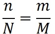
We found the same percentage of natural and artificial errors. Hence the number of errors in the program: The

number of undetected errors is equal to (Nn).
For example, let 20 artificial errors be introduced into the program; during the testing, 12 artificial and 7 natural errors were detected. We get the following estimate of the number of errors in the program: The

number of undetected errors is (Nn) = 12 - 7 = 5.
It is easy to see that there is one significant drawback in the Mills method described above. If we find 100% artificial errors, this will mean that we found 100% of natural errors. But the less we make artificial mistakes, the greater the likelihood that we will find them all. We will introduce the only artificial error, find it, and on this basis we will announce that we have found all natural errors! To solve this problem, Mills added the second part of the model, designed to test the hypothesis about the value of N:
Suppose that the program has N natural errors. We introduce M artificial errors into it . We will test the program until we find all the artificial errors. Let by this moment n be foundnatural mistakes. Based on these numbers, we calculate the value of C :
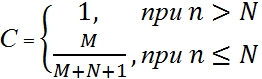
The value of C expresses a measure of confidence in the model. This is the likelihood that the model will correctly reject the false assumption. For example, let us consider that there are no natural errors in the program (N = 0). We introduce 4 artificial errors into the program. We will test the program until we find all the artificial errors. Suppose that we do not find a single natural error. In this case, the measure of confidence in our assumption (that there are no errors in the program) will be 80% (4 / (4 + 0 + 1)). In order to bring it up to 90%, the number of artificial errors will have to be raised to 9. The next 5% confidence in the absence of natural errors will cost us 10 additional artificial errors. M will have to be brought to 19.
If we assume that the program has no more than 3 natural errors (N = 3), add 6 artificial errors (M = 6) to it, find all artificial ones, and one, two or three (but no more!) Natural ones, then the measure confidence in the model will be 60% (6 / (6 + 3 + 1)).
The values of the function C for various values of N and M, in percent:
Table 1 - with step 1;
Table 2 - in increments of 5;
From the formulas for calculating the confidence measure, it is easy to obtain a formula for calculating the number of artificial errors that must be entered into the program to obtain the necessary confidence in the resulting estimate:

The number of artificial errors that must be made to the program to achieve the desired confidence measure for various values of N:
Table 3 - in increments of 1;
Table 4- with step 5;
The Mills model is quite simple. Its weak point is the assumption of the equiprobability of finding errors. In order for this assumption to be justified, the procedure for introducing artificial errors must have a certain degree of “intelligence”. Another weak point is the requirement of the second part of the Mills model to find all artificial errors without fail . And this may not happen for a long time, maybe never.
In 1972, IBM supervisor Harlan Mills proposed the following method for estimating the number of errors in a program. Let us have a program. Suppose there are N errors in it . We call them natural . We introduce in it additional M artificialmistakes. Let's test the program. Let n natural errors and m artificial errors be found during testing . Suppose that the probability of detection is the same for natural and artificial errors. Then the ratio holds:
We found the same percentage of natural and artificial errors. Hence the number of errors in the program: The
number of undetected errors is equal to (Nn).
For example, let 20 artificial errors be introduced into the program; during the testing, 12 artificial and 7 natural errors were detected. We get the following estimate of the number of errors in the program: The
number of undetected errors is (Nn) = 12 - 7 = 5.
It is easy to see that there is one significant drawback in the Mills method described above. If we find 100% artificial errors, this will mean that we found 100% of natural errors. But the less we make artificial mistakes, the greater the likelihood that we will find them all. We will introduce the only artificial error, find it, and on this basis we will announce that we have found all natural errors! To solve this problem, Mills added the second part of the model, designed to test the hypothesis about the value of N:
Suppose that the program has N natural errors. We introduce M artificial errors into it . We will test the program until we find all the artificial errors. Let by this moment n be foundnatural mistakes. Based on these numbers, we calculate the value of C :
The value of C expresses a measure of confidence in the model. This is the likelihood that the model will correctly reject the false assumption. For example, let us consider that there are no natural errors in the program (N = 0). We introduce 4 artificial errors into the program. We will test the program until we find all the artificial errors. Suppose that we do not find a single natural error. In this case, the measure of confidence in our assumption (that there are no errors in the program) will be 80% (4 / (4 + 0 + 1)). In order to bring it up to 90%, the number of artificial errors will have to be raised to 9. The next 5% confidence in the absence of natural errors will cost us 10 additional artificial errors. M will have to be brought to 19.
If we assume that the program has no more than 3 natural errors (N = 3), add 6 artificial errors (M = 6) to it, find all artificial ones, and one, two or three (but no more!) Natural ones, then the measure confidence in the model will be 60% (6 / (6 + 3 + 1)).
The values of the function C for various values of N and M, in percent:
Table 1 - with step 1;
Table 2 - in increments of 5;
From the formulas for calculating the confidence measure, it is easy to obtain a formula for calculating the number of artificial errors that must be entered into the program to obtain the necessary confidence in the resulting estimate:
The number of artificial errors that must be made to the program to achieve the desired confidence measure for various values of N:
Table 3 - in increments of 1;
Table 4- with step 5;
The Mills model is quite simple. Its weak point is the assumption of the equiprobability of finding errors. In order for this assumption to be justified, the procedure for introducing artificial errors must have a certain degree of “intelligence”. Another weak point is the requirement of the second part of the Mills model to find all artificial errors without fail . And this may not happen for a long time, maybe never.