Computational methods in optics or how to model electromagnetic processes on different spatial scales

Among the numerical methods used in the design process of modern optical components, usually distinguish two large groups: universal full-wave and approximate. The choice of a specific approach depends on the ratio of the object being modeled to the wavelength and the nature of the propagation of electromagnetic waves.

Full-wave methods based on the direct solution of the wave equations for the components of the electromagnetic field under given boundary conditions are commonly used to develop optical micro- and nanodevices . While for designing macroscopic systems such as focusing lenses, interferometers and monochromators, approximate methods are used. These include, in particular, geometric ray tracing.

In this article, in addition to a brief analysis of two traditional methods, we will talk about a newer approach, called the beam envelope method, and discuss its advantages for computational optics problems.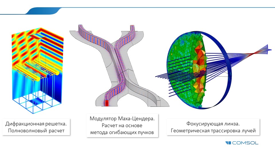

Full wave methods

The first group includes the spectral method, the method of moments, the method of finite differences and the method of finite elements. They have been used successfully for many years and are being actively used at present in the analysis of such important optical components as fiber-optical structures, directional couplers, ring resonators, etc. Using these methods, engineers and researchers can perform an accurate analysis of wave propagation in optical structures using a minimum set of physical assumptions. The latter are associated with discretization when converting a piecewise-continuous optical medium into a digital (discrete) model. Thus, diffraction, interference, and low-order resonance modes can be traced with almost arbitrary precision by simply increasing the discretization level (Fig. 1),

Fig.1. The fall of a plane electromagnetic wave on a gold nanosphere: a picture of a diffused e / m field and a calculated finite element mesh.

In general terms, for finite difference methods, increasing the discretization level is reduced to adding additional points to the computational domain and obtaining a more smooth representation of the electromagnetic field. The same principle applies to other methods. However, a larger number of sampling points leads to an increase in the computational resources required for the calculation. For 3D models, the number of such points is proportional to the wavelength in a cube. According to the Nyquist criterion, the wavelength should be at least two sampling points along each coordinate axis, and in real conditions it should be even longer (usually at least 5 second order elements in each spatial direction). In practice, computational costs grow even faster, so to calculate objects that fit a large number of wavelengths (over 50),

A simple example: the width of an optical fiber can be only a few wavelengths, and its length - several billion wavelengths. For the analysis of modes propagating in the cross section of a fiber, full-wave methods are excellent, since the relative size of the fiber in this direction is small (Fig. 2). On the contrary, to analyze the propagation of waves along the fiber and possible fiber defects, one has to resort to approximate methods in order not to exhaust the computer’s RAM.

Fig. 2. Calculation based on the finite element method of the fiber-optic structure: a finite-element mesh (left) and one of the transverse fiber modes at a wavelength of 1.2 μm (right).

Approximate methods

Approximate methods imply the use of some initial simplifications or approximations. This class of methods includes such methods as ray tracing (or geometric optics ), Gaussian optics, and beam propagation method (BPM) . Unlike the full-wave approach, if certain conditions are met, approximate methods can be applied to solving problems on much larger objects.

For example, in a lens with a diameter of 1 cm, tens of thousands of wavelengths of visible light are placed in any direction. In this case, the optical ray tracing method shows itself best. The price paid for the approximation is the refusal to take into account certain physical phenomena: in geometrical optics, diffraction is usually neglected — rays propagate along straight lines (Fig. 3).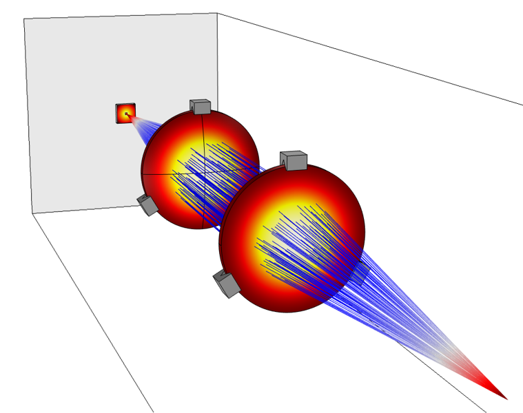

Fig. 3. Numerical analysis of the propagation of electromagnetic waves in a laser beam focusing system is usually based on ray tracing, rather than directly solving the Maxwell equations by the full-wave method.

Beam envelope method

Waveguides in optical systems usually have one preferred direction of wave propagation. In the language of mathematical physics, this means that there is a certain wave vector that changes little or even remains constant in the direction of propagation. This is the basis of a new computational method - the beam envelope method (beam envelope method) .

In the most general case, the electric field of a propagating wave contains three components: $$E = ( E x , E y , E z ) . Suppose that thezaxisis the preferred direction of propagation, and the field inside the waveguide structure oscillates significantly along thezaxisand contains much slower changes in thexandydirections. Then, the field of a continuous electromagnetic wave with a constant frequency can be represented as$$E = E 1 ( x , y , z ) c o s ( w t - k z z ) , where$$w = 2 π f - angular frequency,$$- the propagation constant along the z axis , and$$ - slowly varying amplitude.

This expression is in complex form. $$ can be substituted into the full set of Maxwell's equations and, using a number of classical algebraic transformations, to achieve the reduction of all rapidly changing factors $$getting the final equation for a slowly varying field envelope $$. It is on this successful reduction of the fast-varying component that the beam envelope method is based . To return to the true expression for an electromagnetic wave, it is only necessary to multiply the resulting expression by this factor.

Due to the lack of approximations (the only assumption concerns the initially known direction of wave propagation), this approach can be classified as a full-wave method (Fig. 4), but it also has one important advantage. The problem of the full-wave methods is that they require a sufficient number of calculation points or nodes in the sample, since Otherwise, the results of the calculations will turn out to be simply numerical "garbage". To solve an equation with respect to a slowly varying field envelope, a much smaller number of nodal points is sufficient (while maintaining the Nyquist criterion), at least in cases where the problem has a clearly defined propagation direction, such as in optical waveguides (Fig. 4 ). In this way, The required number of points or sampling nodes can be reduced by an order of magnitude (in some cases even more). It is important to note that to calculate the beam envelope, you can use any universal method, in particular, the FEM, and then to obtain a complete solution, you simply multiply the envelope by the known (initially specified) rapidly changing component.

This approach differs significantly from the method similar in name to the beam propagation method , which uses additional simplifications and approximations, neglecting some derivatives in the wave equation.

Fig. 4. Comparison of the discretization of the traditional full-wave method and the beam envelope method.

The beam envelope method and the direction of wave propagation

The ability to calculate long and thin structures with a more or less constant wave propagation direction is very useful, and it is quite simple to apply the beam envelope method to such cases. However, many waveguide structures are bent in one or several directions. The proposed method will work in this case, but there are some limitations associated with the geometric complexity of the design. If the propagation vector slowly changes its direction, the method remains valid. To understand what is happening in this case, let's return to the full expression for the electromagnetic field.$$where the direction of propagation is initially set along the z axis . To generalize this expression to the case of an arbitrary direction, we write it in the form$$where $$ - the vector that determines the preferred direction of wave propagation, and $$ - vector of coordinates $$ - their scalar product.

In practice, the latter is usually set equal to the spatially distributed phase function. $$. Then, from the point of view of the beam envelope method, the condition of a slowly varying direction of propagation is replaced by the condition of a slowly varying phase. For example, the annular part of the resonator of radius R can be described by the phase function$$where $$ - propagation constant corresponding to the wavelength $$ in the direction of propagation (Fig. 6).

Fig. 6. Analysis of the ring resonator at a wavelength of 1.559 microns. The finite element mesh is shown on the left, the fast-varying physical field is in the center, and the slowly varying envelope of the field, calculated using the beam envelope method, is shown on the right.

Thus, the beam envelope method can be applied to optical structures composed of simple shapes, where each composite component can be described through the function $$corresponding to the preferred local direction of propagation. For example, a ring resonator containing one straight section and one ring section can be examined using one constant and one “circular” phase function. In the more general case, the phase function can be specified as an interpolation of some simple dependence on the coordinate vector. In addition, using the principle of superposition of fields, one can analyze two (forward and backward waves) and more directions of propagation (including tasks with reflection and refraction), recording several sets of phase functions (Fig. 7).

Fig. 7. Distribution of a slowly varying field envelope in a symmetric laser resonator . The calculation uses a superposition of waves (forward and reverse), propagating in two directions.

Application of the beam envelope method in nonlinear optics

Nonlinear optical effects are often quite weak and occur at large interaction lengths, namely, in such cases, the beam envelope method is most appropriate. One example of non-linear effects is self-focusing. This phenomenon can be observed in laser rods or optical glasses located at the focal point (for example, Nd: YAG - an aluminum-yttrium garnet doped with neodymium). Knowing the self-focusing threshold values ​​at the design stage will avoid damage to the materials used in the construction of various elements (Fig. 8).

Fig. 8. Numerical study of self-focusing in a BK-7 rod with a length of 20 cm , i.e. about 300 thousand (!!!) wavelengths. The image on the right is the true aspect ratio, on the left, the scaled visualization of the norm and the z-components of the field envelope.

The method is also applicable to other nonlinear effects: second harmonic generation, total and difference frequency generation, parametric generation and amplification, and also phase self-modulation.

Conclusion

The beam envelope method can significantly increase the size of the models to which the full-wave methods are applicable. It fills the gap between demanding computational resources, but accurate finite difference and finite element schemes and fast ray tracing techniques. The approach is applicable to real-world design problems, which confirms the successful solution of applied problems, both from the field of nonlinear optics and interdisciplinary statements, for example, by calculating Mach-Zehnder modulators .

Developers of the method and its implementation in COMSOL expect that its combination with traditional full-wave and approximate methods will open up new horizons in optics and computational electrodynamics for a comprehensive study of e / m processes on different spatial scales.

PS Additional Information

This article is based on Optik & Photonik magazine materials .

For a more detailed acquaintance with the described techniques, we invite you to participate in our new webinar "Full-wave calculations of extended optical components in COMSOL Multiphysics ^® " , which will be held on November 29, 2017.