Introduction to Convolutional Neural Networks
- Tutorial
The full course in Russian can be found at this link .
The original English course is available at this link .

New lectures are scheduled every 2-3 days.
- So, we are again with Sebastian in the third part of this course. Sebastian, I know that you have done a lot of development using convolutional neural networks. Can you tell us a little more about these networks and what are they? I am sure that the students of our course will listen with no less interest, because in this part they will have to develop the convolutional neural network themselves.
- Well! So, convolutional neural networks are an excellent way of structuring in the network, building the so-called invariance (allocation of immutable features). For example, take the idea of pattern recognition on stage or photograph, you want to understand whether Sebastian is depicted on it or not. It doesn’t matter in which part of the photograph I am located, where my head is located - in the center of the photograph or in the corner. Recognition of my head, my face should occur regardless of where they are located in the image. This is invariance, location variability, which is realized by convolutional neural networks.
- Very interesting! Can you tell us the main tasks in which convolutional neural networks are used?
- Convolutional neural networks are fairly tightly used when working with audio and video, including medical images. They are also used in language technologies, where specialists use deep learning to understand and reproduce language constructions. In fact, there are a lot of applications for this technology, I would even say that they are endless! Her technology can be used in finance and any other areas.
“I used convolutional neural networks to analyze satellite images.”
- Great! The standard task!
- What do you think, can we consider convolutional neural networks as something the last and most advanced tool in the development of deep learning?
- Ha! I have already learned to never say never. There will always be something new and amazing!
“So we still have work to do?” :)
- There will be enough work!
- Fine! In this course, we are just teaching future machine learning pioneers. Do you have any wishes for our students before they start building their first convolutional neural network?
- Here is an interesting fact for you. Convolutional neural networks were invented in 1989, and this is a very long time ago! Most of you were not even born at that time, which means that it’s not the genius of the algorithm that matters, but the data that the algorithm operates on. We live in a world where there is plenty of data to analyze and search for patterns. We have the ability to emulate the functions of the human mind using this huge amount of data. When you work on convolutional neural networks, try to focus on finding the right data and applying them - see what happens and sometimes it can turn out to be real magic, as was the case in our case when we were solving the problem of detecting skin cancer.
- Great! Well, let's finally get down to magic!
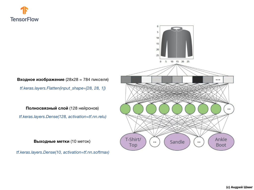
In the last lesson, we learned how to develop deep neural networks that are able to classify images of clothing elements from the Fashion MNIST data set.
The results we achieved while working on the neural network were impressive - 88% classification accuracy. And this is in a few lines of code (not taking into account the code for constructing graphs and images)!
We also experimented with the effect of the number of neurons in hidden layers and the number of training iterations on the accuracy of the model. But how do we make this model even better and more accurate? One way to achieve this is to use convolutional neural networks, abbreviated SNA. SNA show greater accuracy in solving the problems of image classification than the standard fully-connected neural networks that we encountered in previous classes. It is for this reason that the SNA became so popular and it was thanks to them that a technological breakthrough in the field of machine vision became possible.
In this lesson, we will learn how easy it is to develop a SNA classifier from scratch using TensorFlow and Keras. We will use the same Fashion MNIST dataset that we used in the previous lesson. At the end of this lesson, we compare the accuracy of the classification of clothing elements of the previous neural network with the convolutional neural network from this lesson.
Before you dive into the development, it’s worth a little deeper into the working principle of convolutional neural networks.
Two basic concepts in convolutional neural networks:
Let's take a closer look at them.
In this part of our lesson, we will learn a technique called convolution. Let's see how it works.
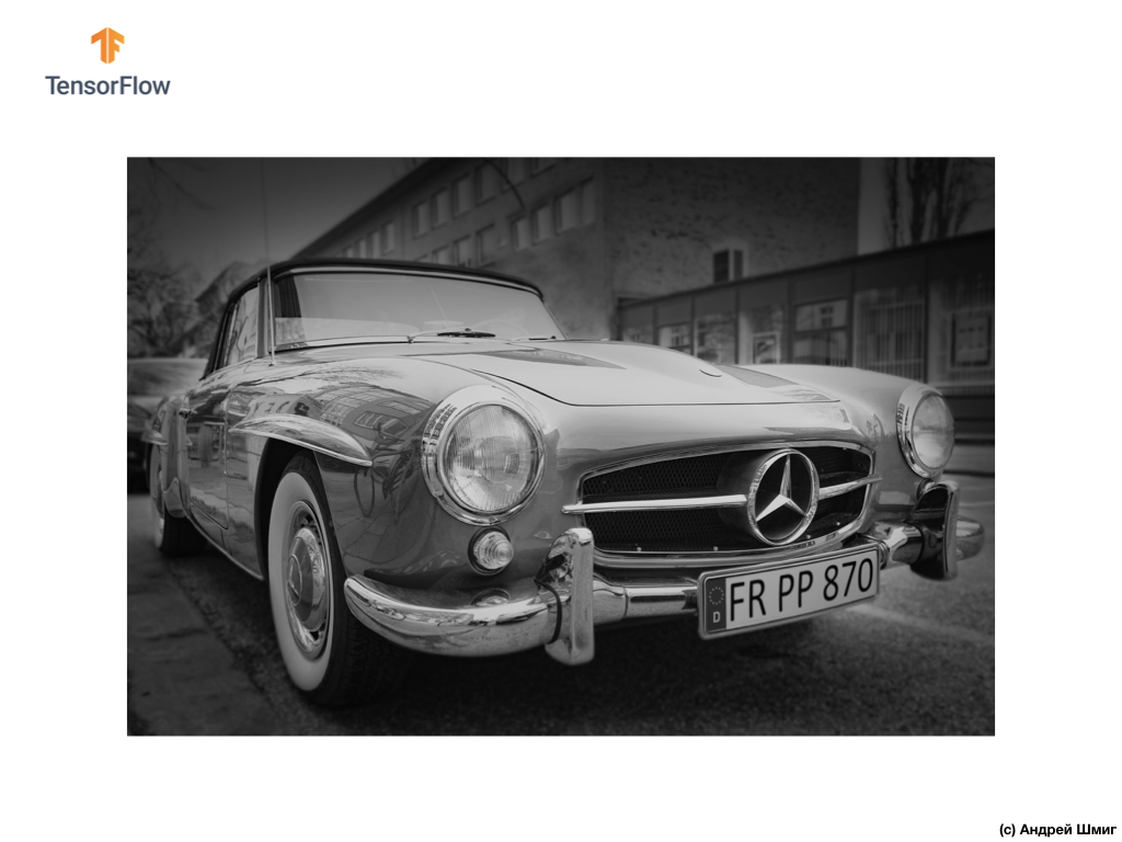
Take an image in shades of gray and, for example, imagine that its dimensions are 6 px in height and 6 px in width.
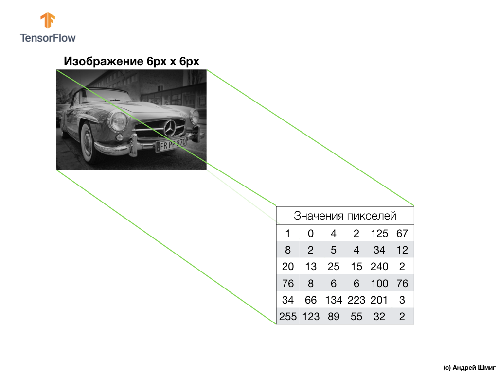
Our computer interprets the image as a two-dimensional array of pixels. Since our image is in shades of gray, the value of each pixel will be in the range from 0 to 255. 0 - black, 255 - white.
In the image below we see a representation of the 6px x 6px image and the corresponding pixel values:
As you already know, before working with images, you need to normalize the pixel values - bring the values to an interval from 0 to 1. However, in this example, for the convenience of explanation, we will save the pixel values of the image and will not normalize them.
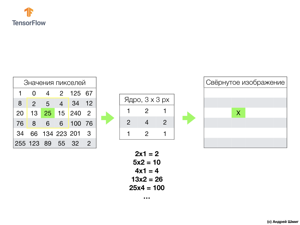
The essence of the convolution is to create another set of values, which is called the kernel or filter. An example can be seen in the image below - a 3 x 3 matrix:

Then we can scan our image using the kernel. The dimensions of our image are 6x6px, and the cores are 3x3px. The convolutional layer is applied to the core and each section of the input image.
Let's imagine that we want to convolution over a pixel with a value of 25 (3 row, 3 column) and the first thing that needs to be done is to center the core over this pixel:

In the image, the core placement is highlighted in yellow. Now we will look only at those pixel values that are in our yellow rectangle, the sizes of which correspond to the sizes of our convolution core.
Now we take the pixel values of the image and the kernel, multiply each pixel of the image with the corresponding pixel of the kernel and add all the product values, and assign the resulting pixel value to the new image.


We perform a similar operation with all the pixels in our image. But what should happen to the pixels at the borders?
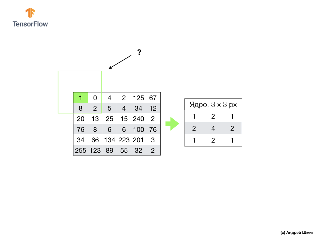
There are several solutions. Firstly, we can simply ignore these pixels, but in this case we will lose information about the image, which may turn out to be significant, and the minimized image will become smaller than the original. Secondly, we can simply "kill" with zero values those pixels whose core values are beyond the scope of the image. The process is called alignment.
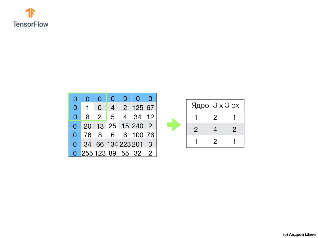
Now that we have made the alignment with zero pixel values, we can calculate the value of the final pixel in the minimized image as before.
A convolution is the process of applying a core (filter) to each part of the input image, by analogy with a fully connected layer (dense layer) we will see that the convolution is the same layer in Keras.
Now let's look at the second concept of convolutional neural networks - the operation of subsampling (pooling, max-pooling).
Now we will consider the second fundamental concept underlying convolutional neural networks - the operation of subsampling (pooling, max-pooling). In simple words, a subsampling operation is the process of compressing (downsizing) an image by adding the values of the blocks of pixels. Let's look at how this works on a concrete example.

To perform the subsampling operation, we need to decide on two components of this process - the sample size (the size of the rectangular grid) and the step size. In this example, we will use a 3x3 rectangular grid and step 3. The step determines the number of pixels by which the rectangular grid should be shifted when performing the subsampling operation.
After we have decided on the grid size and step size, we need to find the maximum pixel value that falls into the selected grid. In the example above, the values 1, 0, 4, 8, 2, 5, 20, 13, 25 fall into the grid. The maximum value is 25. This value is “transferred” to the new image. The grid is shifted 3 pixels to the right and the process of selecting the maximum value and transferring it to a new image is repeated.

As a result, a smaller image will be obtained compared to the original input image. In our example, an image was obtained that is half the size of our original image. The size of the final image will vary depending on the choice of the size of the rectangular grid and step size.
Let's see how this will work in Python!
We became familiar with such concepts as convolution and max-pooling operation.
Convolution is the process of applying a filter (“core”) to an image. The operation of subsampling by maximum value is the process of reducing the size of an image by combining a group of pixels into a single maximum value from this group.
As we will see in the practical part, the convolutional layer can be added to the neural network using the
Some terms that we managed to come across:
We were circled around a finger! It makes sense to perform this practical part only after the previous part has been completed - all the code, except for one block, remains the same. The structure of our neural network is changing, and these are four additional lines for convolutional neural layers and layers of subsampling at the maximum value (max-pooling).
All the detailed explanations of how to work, they promise to give us in the next part - 4 parts.
Oh yes. The accuracy of the model at the training stage became equal to 97% (the model "retrained" at
In this part of the lesson, we studied a new type of neural network - convolutional neural network. We became familiar with such terms as “convolution” and “max-pooling operation”, developed and trained a convolutional neural network from scratch. As a result, we saw that our convolutional neural network produces more accuracy than the neural network that we developed in the last lesson.
PS Note from the author of the translation.
The course is called "Introduction to deep learning using TensorFlow", so we will not complain about the lack of detailed explanations of the principle of convolutional neural networks (layers) - the next two articles will be about the principle of operation of the convolutional neural network and their internal structure (articles do not relate to the course, but were recommended by StackOverflow participants for a better understanding of what is happening).
... and standard call-to-action - sign up, put plus and share :)
YouTube
Telegram
VKontakte
The original English course is available at this link .
New lectures are scheduled every 2-3 days.
Interview with Sebastian
- So, we are again with Sebastian in the third part of this course. Sebastian, I know that you have done a lot of development using convolutional neural networks. Can you tell us a little more about these networks and what are they? I am sure that the students of our course will listen with no less interest, because in this part they will have to develop the convolutional neural network themselves.
- Well! So, convolutional neural networks are an excellent way of structuring in the network, building the so-called invariance (allocation of immutable features). For example, take the idea of pattern recognition on stage or photograph, you want to understand whether Sebastian is depicted on it or not. It doesn’t matter in which part of the photograph I am located, where my head is located - in the center of the photograph or in the corner. Recognition of my head, my face should occur regardless of where they are located in the image. This is invariance, location variability, which is realized by convolutional neural networks.
- Very interesting! Can you tell us the main tasks in which convolutional neural networks are used?
- Convolutional neural networks are fairly tightly used when working with audio and video, including medical images. They are also used in language technologies, where specialists use deep learning to understand and reproduce language constructions. In fact, there are a lot of applications for this technology, I would even say that they are endless! Her technology can be used in finance and any other areas.
“I used convolutional neural networks to analyze satellite images.”
- Great! The standard task!
- What do you think, can we consider convolutional neural networks as something the last and most advanced tool in the development of deep learning?
- Ha! I have already learned to never say never. There will always be something new and amazing!
“So we still have work to do?” :)
- There will be enough work!
- Fine! In this course, we are just teaching future machine learning pioneers. Do you have any wishes for our students before they start building their first convolutional neural network?
- Here is an interesting fact for you. Convolutional neural networks were invented in 1989, and this is a very long time ago! Most of you were not even born at that time, which means that it’s not the genius of the algorithm that matters, but the data that the algorithm operates on. We live in a world where there is plenty of data to analyze and search for patterns. We have the ability to emulate the functions of the human mind using this huge amount of data. When you work on convolutional neural networks, try to focus on finding the right data and applying them - see what happens and sometimes it can turn out to be real magic, as was the case in our case when we were solving the problem of detecting skin cancer.
- Great! Well, let's finally get down to magic!
Introduction
In the last lesson, we learned how to develop deep neural networks that are able to classify images of clothing elements from the Fashion MNIST data set.
The results we achieved while working on the neural network were impressive - 88% classification accuracy. And this is in a few lines of code (not taking into account the code for constructing graphs and images)!
model = tf.keras.Sequential([
   tf.keras.layers.Flatten(input_shape=(28, 28, 1)),
   tf.keras.layers.Dense(128, activation=tf.nn.relu),
   tf.keras.layers.Dense(10, activation=tf.nn.softmax)
])
model.compile(optimizer='adam',
                      loss='sparse_categorical_crossentropy',
                      metrics=['accuracy'])
NUM_EXAMPLES = 60000
train_dataset = train_dataset.repeat().shuffle(NUM_EXAMPLES).batch(32)
test_dataset = test_dataset.batch(32)
model.fit(train_dataset, epochs=5, steps_per_epoch=math.ceil(num_train_examples/32))
test_loss, test_accuracy = model.evaluate(test_dataset, steps=math.ceil(num_test_examples/32))
print('Точность: ', test_accuracy)
Точность: 0.8782
We also experimented with the effect of the number of neurons in hidden layers and the number of training iterations on the accuracy of the model. But how do we make this model even better and more accurate? One way to achieve this is to use convolutional neural networks, abbreviated SNA. SNA show greater accuracy in solving the problems of image classification than the standard fully-connected neural networks that we encountered in previous classes. It is for this reason that the SNA became so popular and it was thanks to them that a technological breakthrough in the field of machine vision became possible.
In this lesson, we will learn how easy it is to develop a SNA classifier from scratch using TensorFlow and Keras. We will use the same Fashion MNIST dataset that we used in the previous lesson. At the end of this lesson, we compare the accuracy of the classification of clothing elements of the previous neural network with the convolutional neural network from this lesson.
Before you dive into the development, it’s worth a little deeper into the working principle of convolutional neural networks.
Two basic concepts in convolutional neural networks:
- convolution
- subsampling operation (pooling, max pooling)
Let's take a closer look at them.
Convolution
In this part of our lesson, we will learn a technique called convolution. Let's see how it works.
Take an image in shades of gray and, for example, imagine that its dimensions are 6 px in height and 6 px in width.
Our computer interprets the image as a two-dimensional array of pixels. Since our image is in shades of gray, the value of each pixel will be in the range from 0 to 255. 0 - black, 255 - white.
In the image below we see a representation of the 6px x 6px image and the corresponding pixel values:
As you already know, before working with images, you need to normalize the pixel values - bring the values to an interval from 0 to 1. However, in this example, for the convenience of explanation, we will save the pixel values of the image and will not normalize them.
The essence of the convolution is to create another set of values, which is called the kernel or filter. An example can be seen in the image below - a 3 x 3 matrix:
Then we can scan our image using the kernel. The dimensions of our image are 6x6px, and the cores are 3x3px. The convolutional layer is applied to the core and each section of the input image.
Let's imagine that we want to convolution over a pixel with a value of 25 (3 row, 3 column) and the first thing that needs to be done is to center the core over this pixel:
In the image, the core placement is highlighted in yellow. Now we will look only at those pixel values that are in our yellow rectangle, the sizes of which correspond to the sizes of our convolution core.
Now we take the pixel values of the image and the kernel, multiply each pixel of the image with the corresponding pixel of the kernel and add all the product values, and assign the resulting pixel value to the new image.
We perform a similar operation with all the pixels in our image. But what should happen to the pixels at the borders?
There are several solutions. Firstly, we can simply ignore these pixels, but in this case we will lose information about the image, which may turn out to be significant, and the minimized image will become smaller than the original. Secondly, we can simply "kill" with zero values those pixels whose core values are beyond the scope of the image. The process is called alignment.
Now that we have made the alignment with zero pixel values, we can calculate the value of the final pixel in the minimized image as before.
A convolution is the process of applying a core (filter) to each part of the input image, by analogy with a fully connected layer (dense layer) we will see that the convolution is the same layer in Keras.
Now let's look at the second concept of convolutional neural networks - the operation of subsampling (pooling, max-pooling).
Subsampling operation (pooling, max-pooling)
Now we will consider the second fundamental concept underlying convolutional neural networks - the operation of subsampling (pooling, max-pooling). In simple words, a subsampling operation is the process of compressing (downsizing) an image by adding the values of the blocks of pixels. Let's look at how this works on a concrete example.
To perform the subsampling operation, we need to decide on two components of this process - the sample size (the size of the rectangular grid) and the step size. In this example, we will use a 3x3 rectangular grid and step 3. The step determines the number of pixels by which the rectangular grid should be shifted when performing the subsampling operation.
After we have decided on the grid size and step size, we need to find the maximum pixel value that falls into the selected grid. In the example above, the values 1, 0, 4, 8, 2, 5, 20, 13, 25 fall into the grid. The maximum value is 25. This value is “transferred” to the new image. The grid is shifted 3 pixels to the right and the process of selecting the maximum value and transferring it to a new image is repeated.
As a result, a smaller image will be obtained compared to the original input image. In our example, an image was obtained that is half the size of our original image. The size of the final image will vary depending on the choice of the size of the rectangular grid and step size.
Let's see how this will work in Python!
Summary
We became familiar with such concepts as convolution and max-pooling operation.
Convolution is the process of applying a filter (“core”) to an image. The operation of subsampling by maximum value is the process of reducing the size of an image by combining a group of pixels into a single maximum value from this group.
As we will see in the practical part, the convolutional layer can be added to the neural network using the
Conv2Dβ-layer in Keras. This layer is similar to the Dense layer, and contains weights and offsets that undergo optimization (selection). Conv2D-the layer also contains filters ("kernels"), the values of which are also optimized. So, in the Conv2D-layer of the value inside the filter matrix there are variables that undergo optimization. Some terms that we managed to come across:
- SNS - convolutional neural networks. A neural network that contains at least one convolutional layer. A typical SNA contains other layers, such as sample layers and fully connected layers.
- Convolution is the process of applying a filter (“core”) to an image.
- A filter (core) is a matrix that is smaller in size than the input data, intended for converting input data in blocks.
- Alignment is the process of adding, most often zero values, to the edges of an image.
- Subsampling operation is the process of reducing the size of an image through sampling. There are several types of subsampling layers, for example, an averaged subsampling layer (sampling an average value), however, a subsampling by the maximum value is most often used.
- The subsampling by the maximum value is the subsampling process, during which many values are converted to a single value - the maximum among the sampling.
- Step - the number of pixels of displacement by the filter (core) in the image.
- Sampling (downsampling) - the process of reducing the size of the image.
CoLab: classification of Fashion MNIST clothing elements using a convolutional neural network
We were circled around a finger! It makes sense to perform this practical part only after the previous part has been completed - all the code, except for one block, remains the same. The structure of our neural network is changing, and these are four additional lines for convolutional neural layers and layers of subsampling at the maximum value (max-pooling).
model = tf.keras.Sequential([
    tf.keras.layers.Conv2D(32, (3,3), padding='same', activation=tf.nn.relu,
                           input_shape=(28, 28, 1)),
    tf.keras.layers.MaxPooling2D((2, 2), strides=2),
    tf.keras.layers.Conv2D(64, (3,3), padding='same', activation=tf.nn.relu),
    tf.keras.layers.MaxPooling2D((2, 2), strides=2),
    tf.keras.layers.Flatten(),
    tf.keras.layers.Dense(128, activation=tf.nn.relu),
    tf.keras.layers.Dense(10,  activation=tf.nn.softmax)
])
All the detailed explanations of how to work, they promise to give us in the next part - 4 parts.
Oh yes. The accuracy of the model at the training stage became equal to 97% (the model "retrained" at
epochs=10), and when running through the data set for the tests, it showed exactly 91%. A noticeable increase in accuracy relative to the previous architecture, where we used only fully connected layers - 88%.Summary
In this part of the lesson, we studied a new type of neural network - convolutional neural network. We became familiar with such terms as “convolution” and “max-pooling operation”, developed and trained a convolutional neural network from scratch. As a result, we saw that our convolutional neural network produces more accuracy than the neural network that we developed in the last lesson.
PS Note from the author of the translation.
The course is called "Introduction to deep learning using TensorFlow", so we will not complain about the lack of detailed explanations of the principle of convolutional neural networks (layers) - the next two articles will be about the principle of operation of the convolutional neural network and their internal structure (articles do not relate to the course, but were recommended by StackOverflow participants for a better understanding of what is happening).
... and standard call-to-action - sign up, put plus and share :)
YouTube
Telegram
VKontakte