Creating a mosaic picture
Surely you have repeatedly seen such pictures on the Internet:
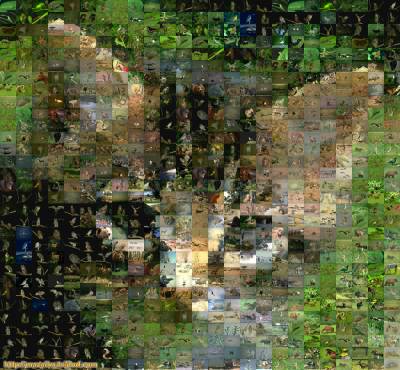
I decided to write a universal script for creating such images.
Let's talk a little about how we are going to do all this. Suppose that there is some limited set of images with which we can pave the canvas, as well as one image, which must be presented in the form of a mosaic. Then we need to split the image that needs to be converted into identical areas, each of which is then replaced with an image from a dataset with pictures.
This raises the question of how to understand which image from the dataset we should replace a certain area. Of course, the ideal tiling of a certain area will be the same area. Each area sized can set
  numbers (here, each pixel corresponds to three numbers - its R, G and B components). In other words, each region is defined by a three-dimensional tensor. Now it becomes clear that to determine the quality of tiling the area with a picture, provided that their sizes coincide, we need to calculate some loss function. In this problem, we can consider the MSE of two tensors:
Here - the number of signs, in our case .
However, this formula does not apply to real cases. The fact is that when the dataset is quite large, and the areas into which the original image is divided are quite small, you will have to do an unacceptably many actions, namely, compress each image from the dataset to the size of the area and consider MSE bycharacteristics. More precisely, in this formula the bad thing is that we are forced to compress absolutely every image for comparison, more than once, but a number equal to the number of areas into which the original picture is divided.
I propose the following solution to the problem: we will sacrifice a little quality and now we will characterize each image from the dataset with only 3 numbers: average RGB in the image. Of course, several problems arise from this: firstly, now the ideal tiling of an area is not only itself, but, for example, it is also upside down (it is obvious that this tiling is worse than the first), and secondly, after calculating the average color, we we can get such R, G and B that the image will not even have a pixel with such components (in other words, it’s difficult to say that our eye perceives the image as a mixture of all its colors). However, I did not come up with a better way.
It turns out that now we can only once calculate the average RGB for images from the dataset, and then use the information received.
Summarizing the above, we find that we now need to select a region that is closest to it from the RGB pixel from the set, and then tile the region with the image from the dataset to which such found medium RGB belongs. To compare the area and the pixel, we will do the same: we transform the area into three numbers and find the closest average RGB. It turns out that we can only find in a set such
  that the Euclidean distance between these two points in three-dimensional space will be minimal:

You can build your own picture dataset. I used to merge datasets with images of lions and dogs .
As I wrote above, we can once calculate the average RGB values for images from the dataset and just save them. What we do:
This script will be executed for a relatively long time, after which the information we need will be saved in the data.pickle file.
Finally, let's move on to creating the mosaic. First, we will write the necessary import s, and also declare several constants:
We get the saved data from the file:
We describe the loss function:
Open the original image:
Now note that tiling is possible if and only if where
where  - the size of the original image, and
  - dimensions of the tiling area. Of course, the above condition is not always satisfied. Therefore, we will crop the original image to suitable sizes, subtracting from the image size their residues from dividing by the size of the region:
Now we proceed directly to the tiling:
Here, in the penultimate line, the desired image area is selected, and in the last line its average RGB components are considered.
Now consider one of the most important lines:
This line sorts all the images of the dataset in ascending order by the value of the loss function for them and gets argmin.
Now we just have to crop the image and replace the area with it:
And finally, display the resulting image on the screen:
In general, there are several options for the loss function, each of which is theoretically applicable to this problem. Their quality can only be evaluated empirically, what can you do :)
Here are some of my results:
The full source code, the already calculated data.pickle file, as well as the archive with the dataset that I collected, you can see in the repository .
I decided to write a universal script for creating such images.
Theoretical part
Let's talk a little about how we are going to do all this. Suppose that there is some limited set of images with which we can pave the canvas, as well as one image, which must be presented in the form of a mosaic. Then we need to split the image that needs to be converted into identical areas, each of which is then replaced with an image from a dataset with pictures.
This raises the question of how to understand which image from the dataset we should replace a certain area. Of course, the ideal tiling of a certain area will be the same area. Each area sized
can set numbers (here, each pixel corresponds to three numbers - its R, G and B components). In other words, each region is defined by a three-dimensional tensor. Now it becomes clear that to determine the quality of tiling the area with a picture, provided that their sizes coincide, we need to calculate some loss function. In this problem, we can consider the MSE of two tensors:
Here
- the number of signs, in our case . However, this formula does not apply to real cases. The fact is that when the dataset is quite large, and the areas into which the original image is divided are quite small, you will have to do an unacceptably many actions, namely, compress each image from the dataset to the size of the area and consider MSE by
characteristics. More precisely, in this formula the bad thing is that we are forced to compress absolutely every image for comparison, more than once, but a number equal to the number of areas into which the original picture is divided.I propose the following solution to the problem: we will sacrifice a little quality and now we will characterize each image from the dataset with only 3 numbers: average RGB in the image. Of course, several problems arise from this: firstly, now the ideal tiling of an area is not only itself, but, for example, it is also upside down (it is obvious that this tiling is worse than the first), and secondly, after calculating the average color, we we can get such R, G and B that the image will not even have a pixel with such components (in other words, it’s difficult to say that our eye perceives the image as a mixture of all its colors). However, I did not come up with a better way.
It turns out that now we can only once calculate the average RGB for images from the dataset, and then use the information received.
Summarizing the above, we find that we now need to select a region that is closest to it from the RGB pixel from the set, and then tile the region with the image from the dataset to which such found medium RGB belongs. To compare the area and the pixel, we will do the same: we transform the area into three numbers and find the closest average RGB. It turns out that we can only
find in a set such that the Euclidean distance between these two points in three-dimensional space will be minimal: Preprocessing dataset
You can build your own picture dataset. I used to merge datasets with images of lions and dogs .
As I wrote above, we can once calculate the average RGB values for images from the dataset and just save them. What we do:
import os
import cv2
import numpy as np
import pickle
items = {}
# cv2 по умолчанию открывает картинки в BGR, а не RGB, поэтому будем их переводить
for path in os.listdir('dogs_images_dataset'):  # у датасета с собаками есть подпапки, поэтому два цикла
    for file in os.listdir(os.path.join('dogs_images_dataset', path)):
        file1 = os.path.join('dogs_images_dataset', path + '/' + file)
        img = np.array(cv2.cvtColor(cv2.imread(file1), cv2.COLOR_BGR2RGB))
        r = round(img[:, :, 0].mean())
        g = round(img[:, :, 1].mean())
        b = round(img[:, :, 2].mean())
        items[file1] = (r, g, b,)
for file in os.listdir('cats_images_dataset'):  # у датасета с кошками подпапок немного, поэтому все изображения можно вручную сохранить в одну директорию
    file1 = os.path.join('cats_images_dataset', file)
    img = np.array(cv2.cvtColor(cv2.imread(file1), cv2.COLOR_BGR2RGB))
    r = round(img[:, :, 0].mean())
    g = round(img[:, :, 1].mean())
    b = round(img[:, :, 2].mean())
    items[file1] = (r, g, b,)
with open('data.pickle', 'wb') as f:
    pickle.dump(items, f)
This script will be executed for a relatively long time, after which the information we need will be saved in the data.pickle file.
Mosaic
Finally, let's move on to creating the mosaic. First, we will write the necessary import s, and also declare several constants:
import os
import cv2
import pickle
import numpy as np
from math import sqrt
PATH_TO_PICTURE = ''  # путь к директории с исходным изображением
PICTURE = 'picture.png'  # имя файла исходного изображения
VERTICAL_SECTION_SIZE = 7  # размер области по горизонтали в пикселях
HORIZONTAL_SECTION_SIZE = 7  # размер области по вертикали в пикселях
We get the saved data from the file:
with open('data.pickle', 'rb') as f:
    items = pickle.load(f)
We describe the loss function:
def lost_function(r_segm, g_segm, b_segm, arg):
    r, g, b = arg[1]
    return sqrt((r - r_segm) ** 2 + (g - g_segm) ** 2 + (b - b_segm) ** 2)
Open the original image:
file = os.path.join(PATH_TO_PICTURE, PICTURE)
img = np.array(cv2.cvtColor(cv2.imread(file), cv2.COLOR_BGR2RGB))
size = img.shape
x, y = size[0], size[1]
Now note that tiling is possible if and only if
where - the size of the original image, and - dimensions of the tiling area. Of course, the above condition is not always satisfied. Therefore, we will crop the original image to suitable sizes, subtracting from the image size their residues from dividing by the size of the region:img = cv2.resize(img, (y - (y % VERTICAL_SECTION_SIZE), x - (x % HORIZONTAL_SECTION_SIZE)))
size = img.shape
x, y = size[0], size[1]Now we proceed directly to the tiling:
for i in range(x // HORIZONT
AL_SECTION_SIZE):
    for j in range(y // VERTICAL_SECTION_SIZE):
        sect = img[i * HORIZONTAL_SECTION_SIZE:(i + 1) * HORIZONTAL_SECTION_SIZE,
                j * VERTICAL_SECTION_SIZE:(j + 1) * VERTICAL_SECTION_SIZE]
        r_mean, g_mean, b_mean = sect[:, :, 0].mean(), sect[:, :, 1].mean(), sect[:, :, 2].mean()
Here, in the penultimate line, the desired image area is selected, and in the last line its average RGB components are considered.
Now consider one of the most important lines:
current = sorted(items.items(), key=lambda argument: lost_function(r_mean, g_mean, b_mean, argument))[0]This line sorts all the images of the dataset in ascending order by the value of the loss function for them and gets argmin.
Now we just have to crop the image and replace the area with it:
resized = cv2.resize(cv2.cvtColor(cv2.imread(current[0]), cv2.COLOR_BGR2RGB),
                             (VERTICAL_SECTION_SIZE, HORIZONTAL_SECTION_SIZE,))
        img[i * HORIZONTAL_SECTION_SIZE:(i + 1) * HORIZONTAL_SECTION_SIZE,
        j * VERTICAL_SECTION_SIZE:(j + 1) * VERTICAL_SECTION_SIZE] = resized
And finally, display the resulting image on the screen:
img = cv2.cvtColor(img, cv2.COLOR_RGB2BGR)
cv2.imshow('ImageWindow', img)
cv2.waitKey(0)
A little more about the loss function
In general, there are several options for the loss function, each of which is theoretically applicable to this problem. Their quality can only be evaluated empirically, what can you do :)

Conclusion
Here are some of my results:
Open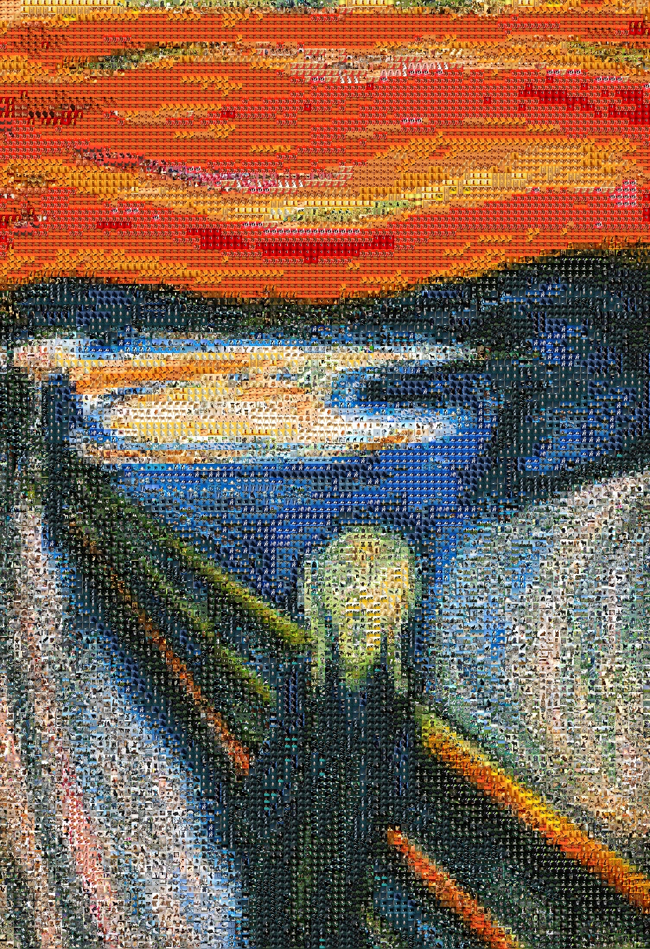
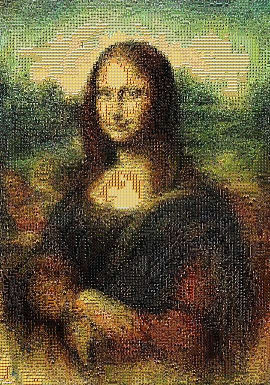
Originals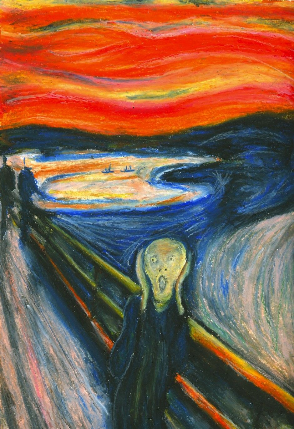
The full source code, the already calculated data.pickle file, as well as the archive with the dataset that I collected, you can see in the repository .