About research of non-stationary processes
It is well known that most of the time series that a researcher has to deal with are non-stationary, and their analysis is significantly more complicated than the study of stationary processes. Since interest in wavelets seems to have subsided, it is useful to discuss some other “non-stationary” instruments, which are primarily suitable for estimating instantaneous frequencies, as well as for evaluating instantaneous spectra.
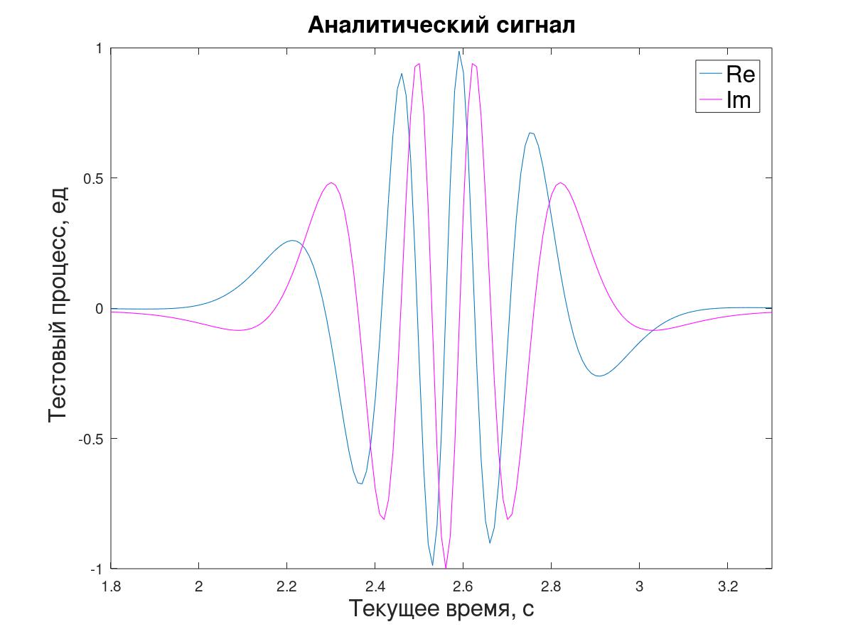
First of all, it makes sense to recall the “analytical signal”. Below, the “An-model" refers to the instantaneous impedance and power of the test signal after completion of its imaginary part (shifted in phase by π / 2).
But it’s not always possible to tinker with the Gilbert transformation. Previously mentionedabout an autoregressive spectral estimation method suitable for working with short sequences. Here, the “AR-model" will be understood as the study of short (from 5 samples) overlapping fragments of the original signal in order to determine the second-order autoregression coefficients, finding the "poles" of the model from them, etc.

Both methods described here are based on one principle - the assumption that in a small neighborhood of the selected time moment the process under study can be approximated by an “exponential” sequence — one complex (An) or the sum of two complex conjugate exponentials (AR).
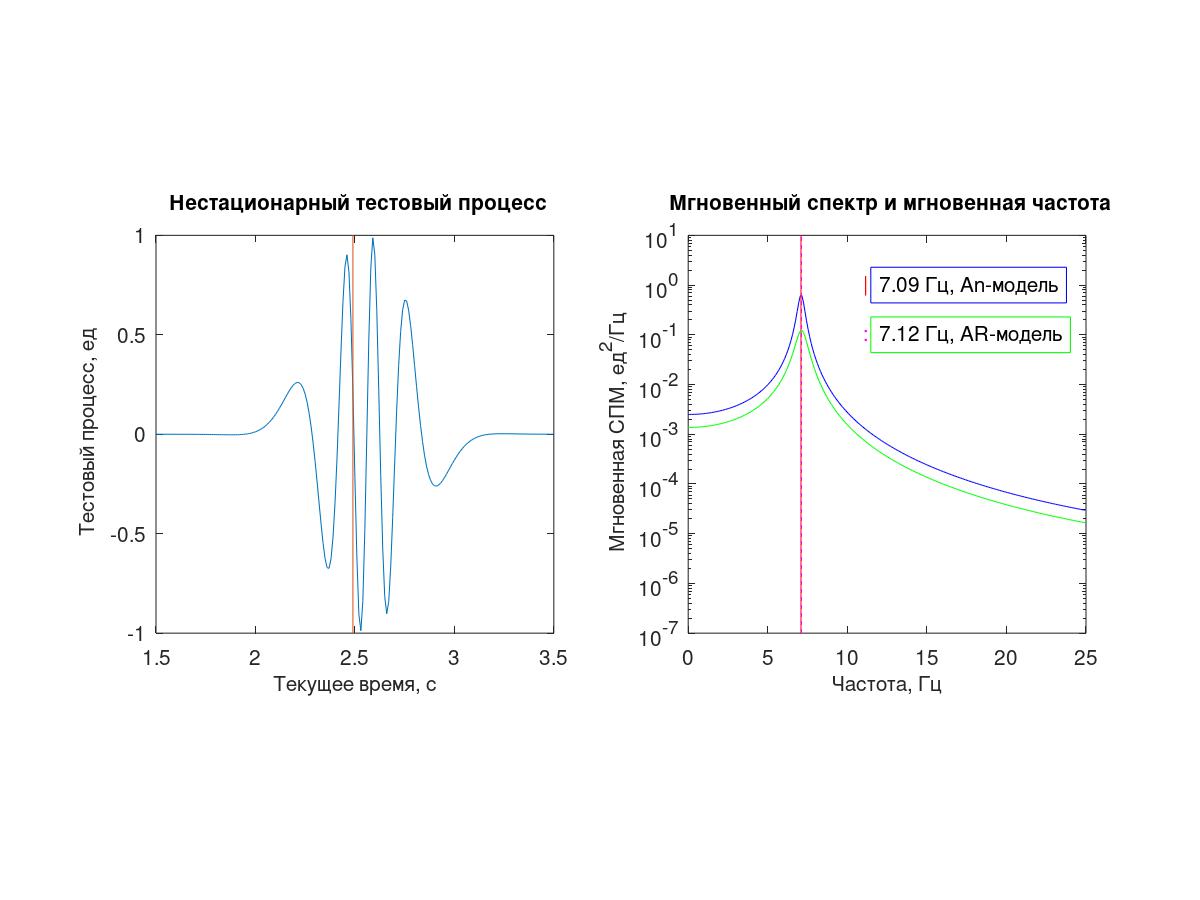
As a test process, a sequence of 512 samples with a conditional sampling interval Δt = 0.01 s, obtained from a continuous deterministic process (1), was used.
By “logarithm” and subsequent differentiation of the high-frequency filling and the envelope from (1), respectively, theoretical expressions for the (instantaneous) frequency and decrement are obtained (2)

For An-modeling by the periodogram method (direct and inverse Fourier transform) from the initial sequence x [i] is formed analytical signal y [i].
The ratio of two consecutive samples of such a signal, in principle, allows you to determine the instantaneous impedance λ, but in order to simplify this demonstration task — so as not to bother with creating intermediate samples or explaining the shift of the estimate by Δt / 2 — it was decided to work with samples “through one”, calculating λ i with respect to the subsequent y [i + 1] signal values to the previous y [i-1] (3).

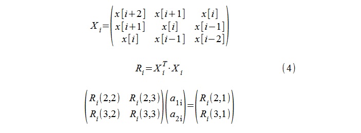
For AR modeling (second-order model), the standard procedure for calculating the autocorrelation coefficients 1, a 1i , a 2i using the Yule-Walker equations was used, and the 5-sample sequences x [i-2], x [i -1], ... x [i + 2] (4).
The “poles” of the model λ ithen they are easily calculated by logarithm of the roots of the quadratic equation (5).


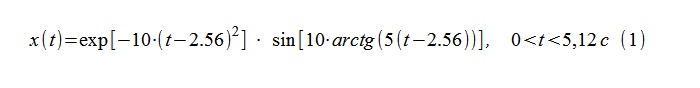
The construction of spectral estimates from the known “poles” up to a scale factor is not difficult . Further. The “instantaneous power” for the An-model is obviously defined as | y [i] | 2, and the question of scaling this estimate seems to be settled. For the AR model, the usual technique associated with determining the power of conventional white noise, in the case of an unsteady signal, “does not work”. For lack of best ideas, scaling was applied based on the average square of the corresponding 5 samples. It seems that nothing more can be done by analyzing only the 5-sample sequence. The animation shows how the SPM AR-chart sometimes noticeably “fails” relative to the An-score. It should be understood that the moments of the “through zero” transition for the AR model can be difficult not only in terms of errors with instantaneous frequency, but also with instantaneous amplitude, especially in the low-frequency region.
A few comments in the end.
First of all, it makes sense to recall the “analytical signal”. Below, the “An-model" refers to the instantaneous impedance and power of the test signal after completion of its imaginary part (shifted in phase by π / 2).
But it’s not always possible to tinker with the Gilbert transformation. Previously mentionedabout an autoregressive spectral estimation method suitable for working with short sequences. Here, the “AR-model" will be understood as the study of short (from 5 samples) overlapping fragments of the original signal in order to determine the second-order autoregression coefficients, finding the "poles" of the model from them, etc.
Both methods described here are based on one principle - the assumption that in a small neighborhood of the selected time moment the process under study can be approximated by an “exponential” sequence — one complex (An) or the sum of two complex conjugate exponentials (AR).
As a test process, a sequence of 512 samples with a conditional sampling interval Δt = 0.01 s, obtained from a continuous deterministic process (1), was used.
By “logarithm” and subsequent differentiation of the high-frequency filling and the envelope from (1), respectively, theoretical expressions for the (instantaneous) frequency and decrement are obtained (2)
For An-modeling by the periodogram method (direct and inverse Fourier transform) from the initial sequence x [i] is formed analytical signal y [i].
The ratio of two consecutive samples of such a signal, in principle, allows you to determine the instantaneous impedance λ, but in order to simplify this demonstration task — so as not to bother with creating intermediate samples or explaining the shift of the estimate by Δt / 2 — it was decided to work with samples “through one”, calculating λ i with respect to the subsequent y [i + 1] signal values to the previous y [i-1] (3).
For AR modeling (second-order model), the standard procedure for calculating the autocorrelation coefficients 1, a 1i , a 2i using the Yule-Walker equations was used, and the 5-sample sequences x [i-2], x [i -1], ... x [i + 2] (4).
The “poles” of the model λ ithen they are easily calculated by logarithm of the roots of the quadratic equation (5).
The construction of spectral estimates from the known “poles” up to a scale factor is not difficult . Further. The “instantaneous power” for the An-model is obviously defined as | y [i] | 2, and the question of scaling this estimate seems to be settled. For the AR model, the usual technique associated with determining the power of conventional white noise, in the case of an unsteady signal, “does not work”. For lack of best ideas, scaling was applied based on the average square of the corresponding 5 samples. It seems that nothing more can be done by analyzing only the 5-sample sequence. The animation shows how the SPM AR-chart sometimes noticeably “fails” relative to the An-score. It should be understood that the moments of the “through zero” transition for the AR model can be difficult not only in terms of errors with instantaneous frequency, but also with instantaneous amplitude, especially in the low-frequency region.
A few comments in the end.
- From experience, both methods usually give good results in estimating the instantaneous frequency, at least in the average (based on the sampling frequency) frequency range.
- The relatively high quality of the results of the An-method, its simplicity and ease of understanding and implementation are more than “compensated” by the possible difficulties with transforming the process according to Gilbert. A Gilbert digital filter of good quality, especially in a wide frequency range, can have an unacceptably high order. When implementing an alternative periodogram method of this transformation, it must be taken into account that the Fourier transform implicitly implies the completion of the process to periodic. As a result, a significant significant completion of the process with zeros may be required. The high quality of the results of the An-method is explained by its use of information on a very vast neighborhood of the selected time instant (strictly speaking - on the entire temporary implementation of the process), and this same property makes it difficult to implement the method (e.g.
- If necessary, the following measures can be recommended to improve the results of the AR method:
- Data thinning (at an excessively high sampling rate)
- An increase in the number of averagings — an extension of the “moment of time” involved in the model of the neighborhood — the construction of a track matrix X with a large number of rows.
- Increasing the order of the AR model.