Classification of land cover using eo-learn. Part 1

Hello, Habr! I present to you the translation of the article " Land Cover Classification with eo-learn: Part 1 " by Matic Lubej.

Part 2
Part 3

Foreword

About six months ago, the first commit was made to the eo-learn repository on GitHub. Today, it eo-learnhas turned into a wonderful open source library, ready for use by anyone who is interested in EO data (Earth Observation - pr. Per.). Everyone in the Sinergise team was waiting for the moment of transition from the stage of building the necessary tools to the stage of their use for machine learning. It's time to introduce you a series of articles regarding the classification of land cover usingeo-learn

eo-learnIs an open source Python library that acts as a bridge connecting Earth Observation / Remote Sensing to the ecosystem of Python machine learning libraries. We already wrote a separate post on our blog , which we recommend that you familiarize yourself with. The library uses the primitives of the libraries numpyand shapelyto store and manipulate data from satellites. At the moment, it is available in the GitHub repository , and the documentation is available at the appropriate link to ReadTheDocs .

Sentinel-2 satellite image and NDVI mask of a small area in Slovenia in winter

To demonstrate the possibilities eo-learn, we decided to use our multi-temporal conveyor to classify the cover of the territory of the Republic of Slovenia (the country where we live), using data for 2017. Since the complete procedure may be too complicated for one article, we decided to divide it into three parts. Thanks to this, there is no need to skip the steps and immediately proceed to machine learning - first we have to really understand the data we work with. Each article will be accompanied by a Jupyter Notebook example. Also, for those interested, we have already prepared a complete example covering all stages.

• In the first article, we will guide you through the procedure for selecting / splitting an area of ​​interest (hereinafter - AOI, area of ​​interest), and obtaining the necessary information, such as data from satellite sensors and cloud masks. We also show an example of how to create a raster mask of data on real coverage of a territory from vector data. All these are necessary steps to obtain a reliable result.
• In the second part, we dive headlong into the preparation of data for the machine learning procedure. This process includes taking random samples for training \ validation of pixels, removing cloud images, interpolating temporal data to fill in “holes”, etc.
• In the third part we will consider the training and validation of the classifier, as well as, of course, beautiful graphics!

Sentinel-2 satellite image and NDVI mask of a small area in Slovenia in summer

Area of ​​interest? Choose!

The library eo-learnallows you to split AOI into small fragments that can be processed in conditions of limited computing resources. In this example, the Slovenian border was taken from Natural Earth , however, you can select a zone of any size. We also added a buffer to the border, after which the AOI dimension was approximately 250x170 km. Using the magic of libraries geopandasand shapely, we created a tool for breaking AOI. In this case, we divided the territory into 25x17 squares of the same size, as a result of which we received ~ 300 fragments of 1000x1000 pixels, in a resolution of 10m. The decision about splitting into fragments is made depending on the available computing power. As a result of this step, we get a list of squares covering the AOI.

AOI (territory of Slovenia) is divided into small squares with a size of approximately 1000x1000 pixels in a resolution of 10m.

Receiving data from Sentinel satellites

After determining the squares, eo-learnit allows you to automatically download data from Sentinel satellites. In this example, we get all the Sentinel-2 L1C images that were taken in 2017. It is worth noting that Sentinel-2 L2A products, as well as additional data sources (Landsat-8, Sentinel-1) can be added to the pipeline in a similar way. It is also worth noting that the use of L2A products can improve the classification results, but we decided to use L1C for the versatility of the solution. This was done using a sentinelhub-pylibrary that works like a wrapper on Sentinel-Hub services. Using these services is free for research institutes and start-ups, but in other cases it is necessary to subscribe.

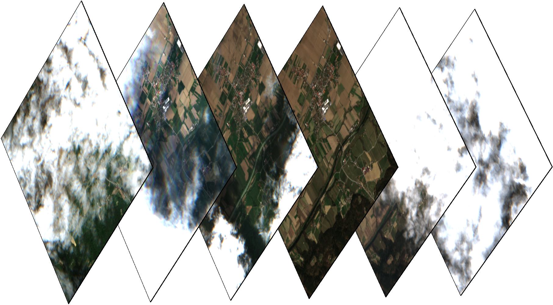
Color images of one fragment on different days. Some images are cloudy, which means a cloud detector is needed.

In addition to Sentinel data, eo-learnit allows you to transparently access cloud and cloud probability data through the library s2cloudless. This library provides tools for automatically detecting clouds pixel by pixel . Details can be read here .

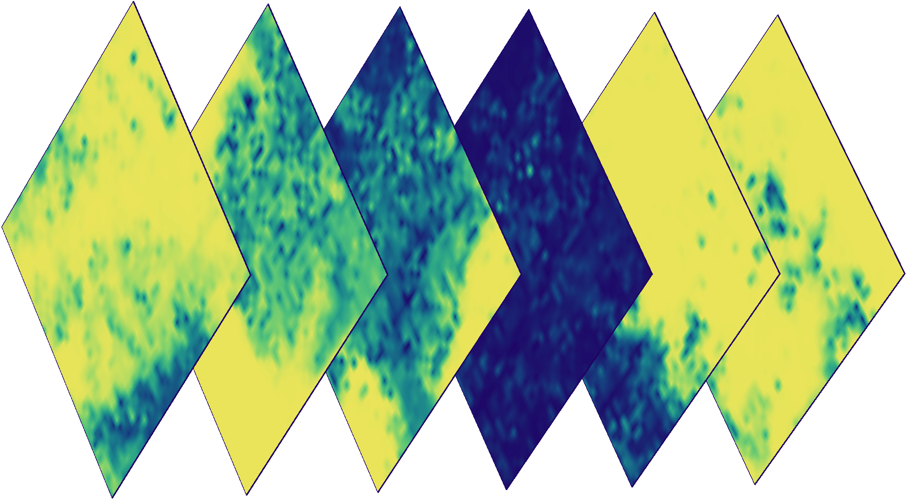
Cloud Masks for the images above. Color indicates the probability of cloudiness of a specific pixel (blue - low probability, yellow - high).

Adding Real Data

Teaching with a teacher requires a card with real data, or truth . The last term should not be taken literally, because in reality, data is only an approximation of what is on the surface. Unfortunately, the behavior of the classifier strongly depends on the quality of this card ( however, as for most other tasks in machine learning ). Marked cards are most often available as vector data in a format shapefile(for example, provided by the state or community ). eo-learncontains tools for rasterizing vector data in the form of a raster mask.

The process of rasterizing data into masks using the example of one square. Polygons in a vector file are shown on the left image, raster masks for each label are shown in the middle - black and white colors indicate the presence and absence of a specific attribute, respectively. The right image shows a combined raster mask in which different colors indicate different labels.

Putting it all together

All these tasks behave like building blocks that can be combined into a convenient sequence of actions performed for each square. Due to the potentially extremely large number of such fragments, pipeline automation is absolutely necessary

# Определим задачу
eo_workflow = eolearn.core.LinearWorkflow(
    add_sentinel2_data, # получение данных со спутника Sentinel-2
    add_cloud_mask, # получение маски вероятности облаков
    append_ndvi, # расчёт NDVI
    append_ndwi, # расчёт NDWI 
    append_norm, # расчёт статистических характеристик изображения
    add_valid_mask, # создание маски присутствия данных
    add_count_valid, # подсчёт кол-ва пикселей с данными в изображении
    *reference_task_array, # добавление масок с метками из референсного файла
    save_task # сохраняем изображения
)

Getting to know the actual data is the first step in working with tasks of this kind. Using cloud masks paired with data from Sentinel-2, you can determine the number of quality observations of all pixels, as well as the average probability of clouds in a particular area. Thanks to this, you can better understand the existing data, and use this when debugging further problems.

Color image (left), mask of the number of quality measurements for 2017 (center), and average cloud cover probability for 2017 (right) for a random fragment from AOI.

Someone might be interested in the average NDVI for an arbitrary zone, ignoring the clouds. Using cloud masks, you can calculate the average value of any feature, ignoring pixels without data. Thus, thanks to the masks, we can clear images from noise for almost any feature in our data.

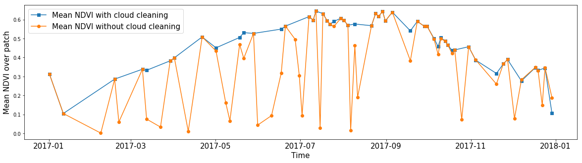
The average NDVI of all pixels in a random AOI fragment throughout the year. The blue line shows the calculation result obtained if ignoring the values ​​inside the clouds. The orange line shows the average value when all pixels are taken into account.

"But what about scaling?"

After we set up our conveyor using an example of one fragment, all that remains to be done is to start a similar procedure for all fragments automatically (in parallel, if resources allow), while you relax with a cup of coffee and think about how big the boss will be pleasantly surprised the results of your work. After the end of the pipeline, you can export the data you are interested in into a single image in GeoTIFF format. The script gdal_merge.py receives the images and combines them, resulting in a picture that covers the whole country.

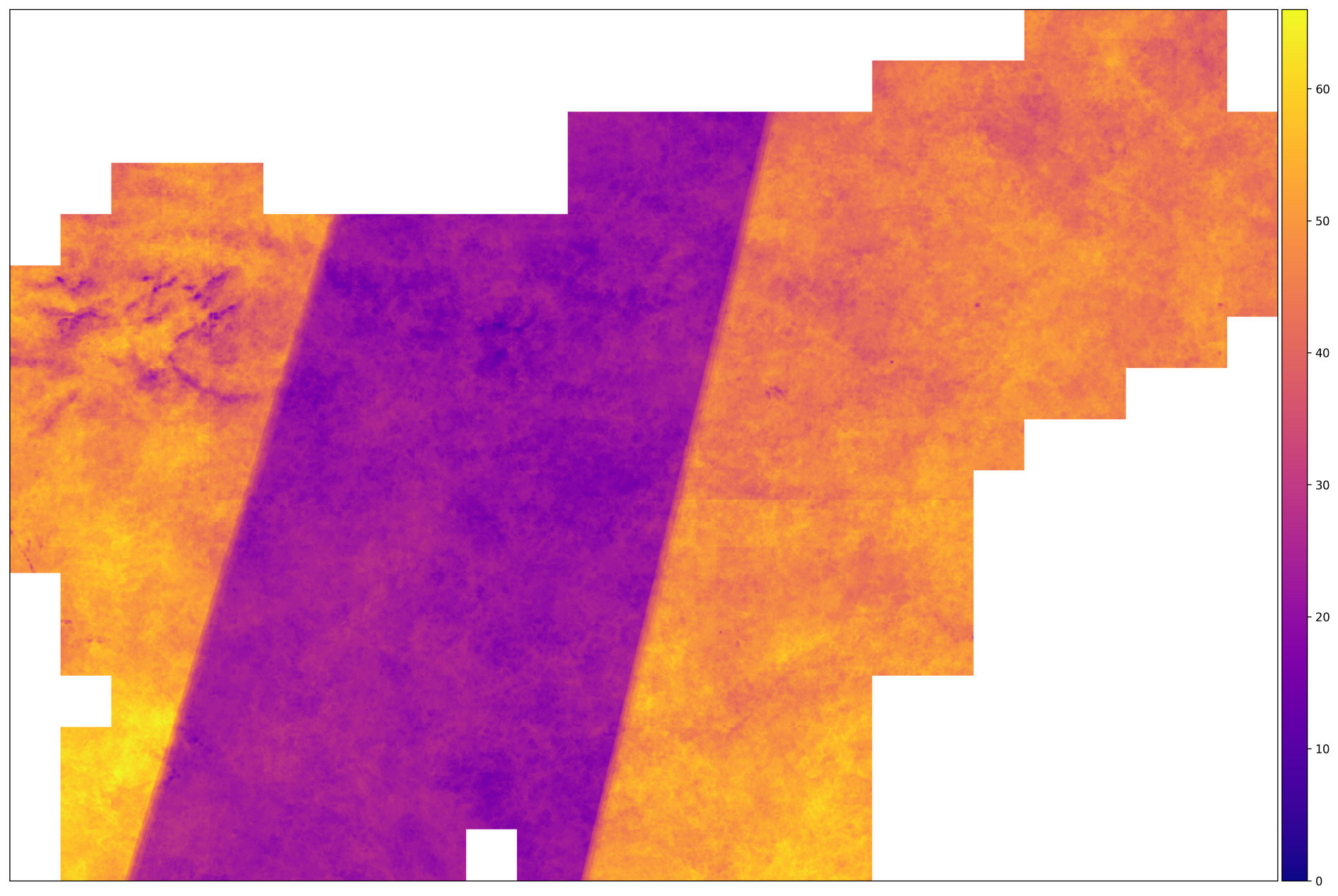
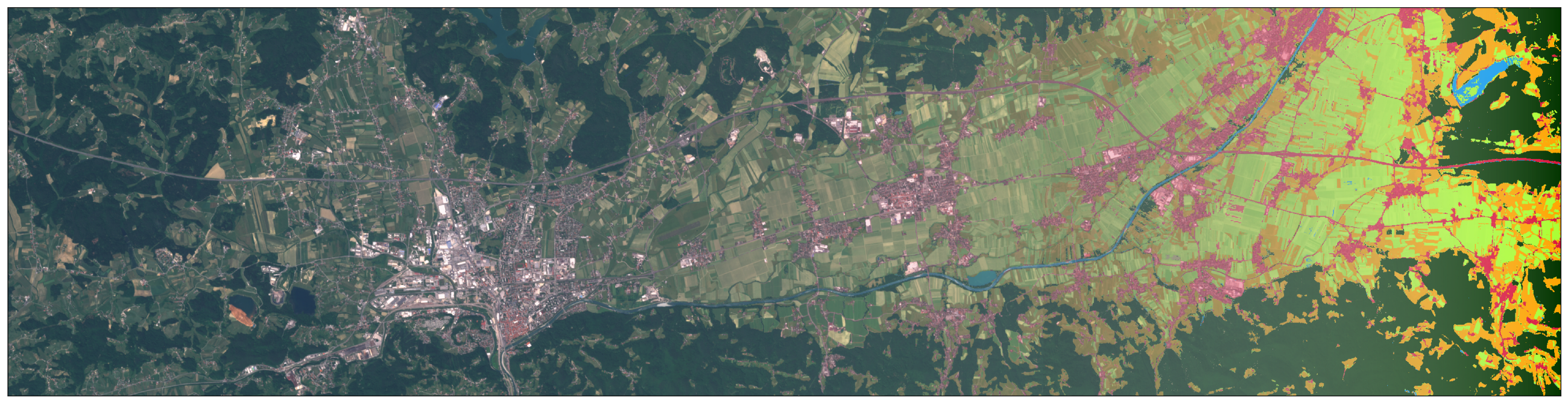
The number of correct shots for AOI in 2017. Regions with a large number of images are located on the territory where the trajectory of the Sentinel-2A and Sentinel-2B satellites intersect. In the middle of this does not happen.

From the image above, we can conclude that the input data is heterogeneous - for some fragments, the number of images is two times higher than for others. This means that we need to take measures to normalize the data - such as interpolation along the time axis.

The execution of the specified pipeline takes approximately 140 seconds for one fragment, which in total gives ~ 12 hours when starting the process throughout the AOI. Most of this time is downloading satellite data. The average uncompressed fragment with the described configuration takes about 3 GB, which in total gives ~ 1 TB of space for the entire AOI.

Example in a Jupyter Notebook

For a simpler introduction to the code, eo-learnwe have prepared an example covering the topics discussed in this post. The example is designed as a Jupyter notepad, and you can find it in the sample package directory eo-learn.