How and why did we do landmark recognition in Mail.ru Cloud

With the advent of high-quality cameras in mobile phones, we are photographing more and more often, shooting videos of the bright and important moments of our lives. Many of us have photo archives dating back tens of years and thousands of photographs, in which it is becoming increasingly difficult to navigate. Remember how long it often took to find the right photo several years ago.
One of the goals of Mail.ru Cloud is to provide the most convenient access and search in your photo and video archive. To do this, we, the Mail.ru machine vision team, have created and implemented smart photo processing systems: search by objects, scenes, faces, etc. Another such striking technology is the recognition of sights. And today I’ll talk about how we solved this problem with the help of Deep Learning.
Imagine the situation: you went on vacation and brought a bunch of photos. And in a conversation with friends, they asked you to show how you visited a palace, castle, pyramid, temple, lake, waterfall, mountain, etc. You start frantically scrolling through the folder with photos, trying to find the right one. Most likely, you do not find it among hundreds of images, and say that you will show later.
We solve this problem by grouping custom photos into albums. This makes it easy to find the right pictures in just a few clicks. Now we have albums on faces, on objects and scenes, as well as on attractions.
Photos with landmarks are important because they often display significant moments of our lives (for example, travel). These can be photographs in the background of some architectural structure or a corner of nature untouched by man. Therefore, we need to find these photos and give users easy and quick access to them.
Feature recognition
But there is a nuance: you can’t just take and train some model to recognize the sights, there are a lot of difficulties.
- Firstly, we cannot clearly describe what a “landmark” is. We can’t say why one building is a landmark, and standing next to it is not. This is not a formalized concept, which complicates the formulation of the recognition problem.
- Secondly, the sights are extremely diverse. It can be historical or cultural buildings - temples, palaces, castles. These can be the most diverse monuments. It can be natural objects - lakes, canyons, waterfalls. And one model must be able to find all these attractions.
- Thirdly, there are very few images with sights, according to our calculations, they are found only in 1-3% of user photos. Therefore, we cannot allow ourselves mistakes in recognition, because if we show a person a photo without a point of interest, it will be immediately noticeable and will cause bewilderment and negative reaction. Or, on the contrary, we showed the person a photo with a landmark in New York, and he had never been to America. So the recognition model must have a low FPR (false positive rate).
- Fourth, about 50% of users, or even more, turn off the storage of geo-information when photographing. We need to take this into account and determine the place solely from the image. Most services that today somehow manage to work with places of interest do this thanks to geodata. Our initial requirements were tougher.
I will show now with examples.
Here are similar objects, three French Gothic cathedrals. The left is the Amiens Cathedral, in the middle of the Reims Cathedral, on the right is Notre Dame de Paris.
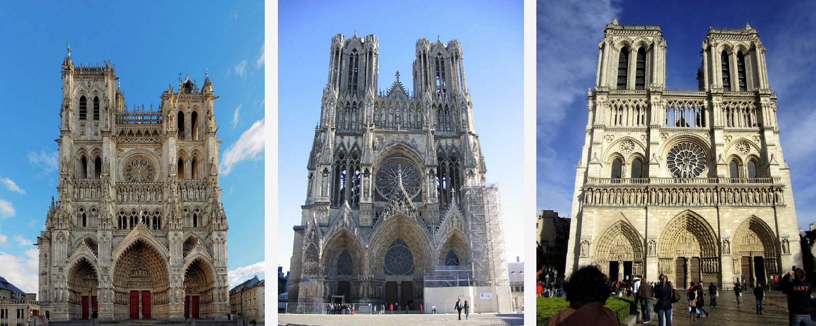
Even a person needs some time to look at them and understand that these are different cathedrals, and the machine must also be able to cope with it, and faster than a person.
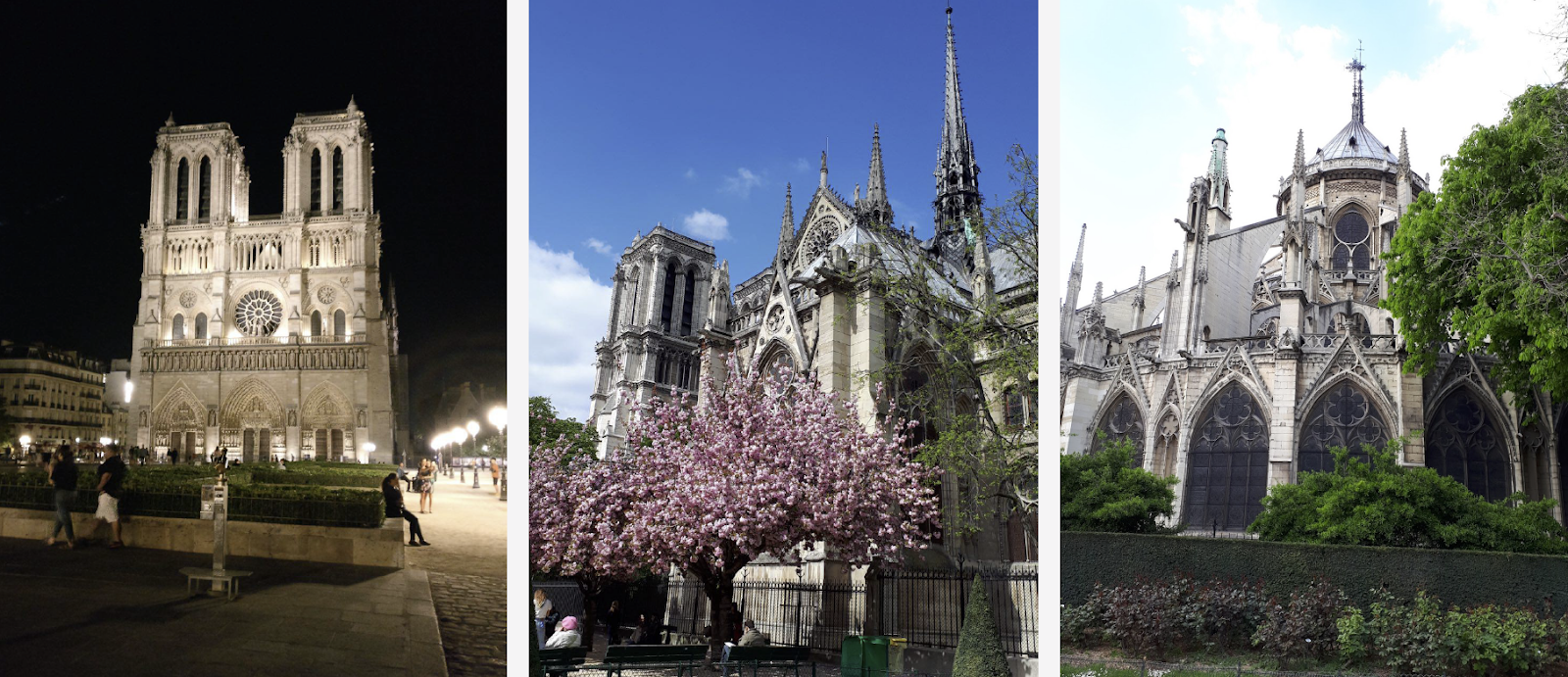
And here is an example of another difficulty: the three photos on the slide are Notre Dame de Paris, taken from different angles. The photos turned out to be very different, but they all need to be recognized and found.
Natural objects are completely different from architectural ones. On the left is Caesarea in Israel, on the right is the English Park in Munich.
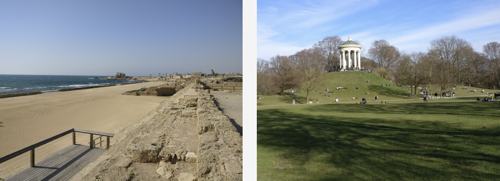
In these photographs there are very few characteristic details for which the model can “catch on”.
Our method
Our method is completely based on deep convolutional neural networks. As an approach to learning, they chose the so-called curriculum learning - learning in several stages. In order to work more efficiently both in the presence of geodata and in the absence thereof, we made a special inference (conclusion). I’ll tell you about each of the stages in more detail.
Datacet
The fuel for machine learning is data. And first of all, we needed to collect a dataset for model training.
We divided the world into 4 regions, each of which is used at different stages of training. Then, countries were taken in each region, for each country a list of cities was compiled and a database of photos of their attractions was compiled. Examples of data are presented below.

First, we tried to train our model on the resulting base. The results were bad. They began to analyze, and it turned out that the data is very "dirty." Each attraction had a large amount of garbage. What to do? Manually reviewing the entire huge amount of data is expensive, dreary and not very smart. Therefore, we did an automatic cleaning of the base, during which manual processing is used only at one step: for each attraction, we manually selected 3-5 reference photographs that accurately contain the desired attraction in a more or less correct perspective. It turns out pretty quickly, because the volume of such reference data is small relative to the entire database. Then, automatic cleaning based on deep convolutional neural networks is already performed.
Further I will use the term "embedding", by which I will understand the following. We have a convolutional neural network, we trained it for classification, cut off the last classification layer, took some images, drove through the network and received a numerical vector at the output. I will call it embedding.
As I said, our training was carried out in several stages, corresponding to parts of our database. Therefore, first we take either a neural network from the previous stage, or an initializing network.
We’ll run the photos of the sights through the network and get several embeddings. Now you can clean the base. We take all the pictures from the dataset for this attraction, and we also drive each picture through the network. We get a bunch of embeddings and for each of them we consider the distances to the embedding of standards. Then we calculate the average distance, and if it is more than a certain threshold, which is the parameter of the algorithm, then we consider that this is not a tourist attraction. If the average distance is less than the threshold, then we leave this photo.
As a result, we got a database that contains more than 11 thousand attractions from more than 500 cities in 70 countries of the world - over 2.3 million photos. Now it's time to remember that most of the photos do not contain attractions at all. This information needs to be somehow shared with our models. Therefore, we added 900 thousand photos without sights to our database, and trained our model on the resulting dataset.
To measure the quality of training, we introduced an offline test. Based on the fact that sights are found only in about 1-3% of photographs, we manually compiled a set of 290 photographs that show sights. These are different, quite complex photographs with a large number of objects taken from different angles, so that the test is as difficult as possible for the model. By the same principle, we selected 11 thousand photographs without sights, which are also quite complex, and we tried to find objects that are very similar to the sights available in our database.
To assess the quality of training, we measure the accuracy of our model from photographs with and without sights. These are our two main metrics.
Existing approaches
There is relatively little information on sight recognition in the scientific literature. Most solutions are based on local features. The idea is that we have a certain request picture and a picture from the database. In these pictures we find local signs - key points, and compare them. If the number of matches is large enough, we think we’ve found a point of interest.
To date, the best method is Google’s proposed method, DELF (deep local features), in which a comparison of local features is combined with deep learning. By running the input image through the convolution network, we get some DELF-signs.

How is the recognition of attractions? We have a database of photos and an input image, and we want to understand if there is a tourist attraction on it or not. We run all the pictures through DELF, we get the corresponding signs for the base and for the input image. Then we perform a search using the method of nearest neighbors and at the output we get candidate images with signs. We compare these signs with the help of geometric verification: if they pass it successfully, then we believe that there is a point of interest in the picture.
Convolutional Neural Network
For Deep Learning, pre-training is crucial. Therefore, we took the base of scenes and pre-trained on it our neural network. Why so? A scene is a complex object that includes a large number of other objects. And the attraction is a special case of the scene. A pre-training model on such a basis, we can give the model an idea of some low-level features that can then be generalized for the successful recognition of attractions.
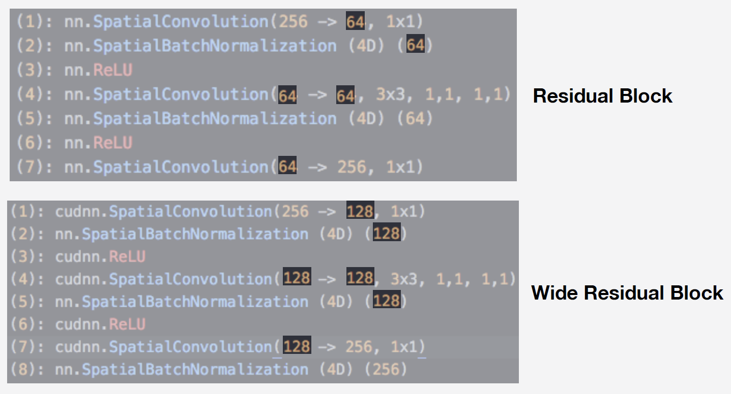
As a model, we used a neural network from the Residual network family. Their main feature is that they use a residual block, which includes a skip connection, which allows the signal to pass freely without getting into layers with weights. With this architecture, you can qualitatively train deep networks and deal with the effect of gradient blur, which is very important when learning.
Our model is Wide ResNet 50-2, a modification of ResNet 50, in which the number of convolutions in the internal bottleneck block is doubled.
The network is very efficient. We conducted tests on our scene database and this is what we got:
| Model | Top 1 err | Top 5 err |
|---|---|---|
| ResNet-50 | 46.1% | 15.7% |
| ResNet-200 | 42.6% | 12.9% |
| SE-ResNext-101 | 42% | 12.1% |
| WRN-50-2 (fast!) | 41.8% | 11.8% |
Wide ResNet turned out to be almost twice as fast as the rather large ResNet 200 network. And the speed of operation is very important for operation. Based on the totality of these circumstances, we took Wide ResNet 50-2 as our main neural network.
Training
To train the network, we need loss (loss function). To select it, we decided to use the metric learning approach: a neural network is trained so that representatives of the same class are pulled together in one cluster. At the same time, clusters for different classes should be as far apart as possible. For attractions, we used Center loss, which pulls together points of the same class to a certain center. An important feature of this approach is that it does not require negative sampling, which in the later stages of training is a rather difficult procedure.
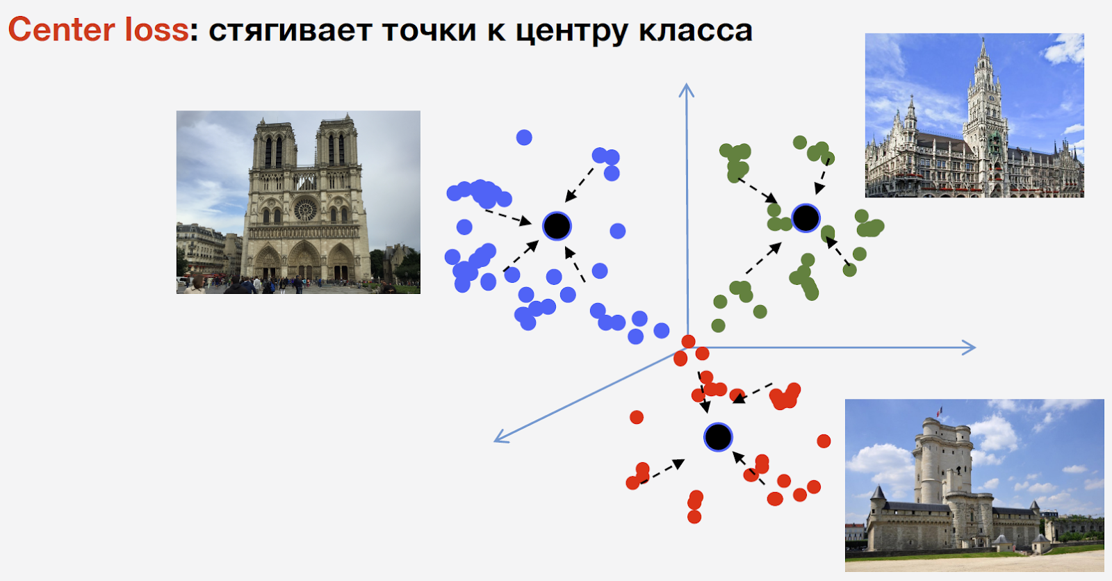
Let me remind you that we have n classes of attractions and another class of “not attractions”, Center loss is not used for it. We mean that a landmark is one and the same object, and there is a structure in it, therefore it is advisable to consider a center for it. But not a tourist attraction can be anything, and to consider the center for him is unreasonable.
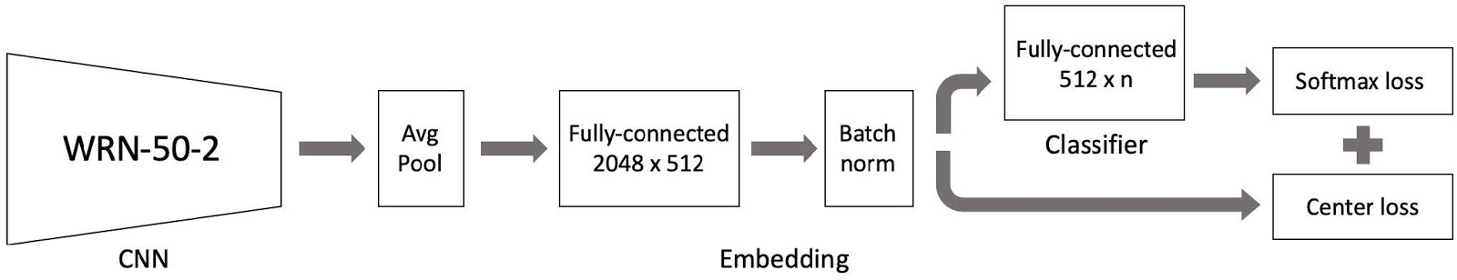
Then we put it all together and got a model for training. It consists of three main parts:
- Convolutional neural network Wide ResNet 50-2, pre-trained on the basis of scenes;
- Parts of embedding consisting of a fully connected layer and a Batch norm layer;
- A classifier, which is a fully connected layer, followed by a pair of Softmax loss and Center loss.
As you remember, our base is divided into 4 parts by region of the world. We use these 4 parts as part of the curriculum learning paradigm. At each stage, we have the current dataset, we add another part of the world to it and we get a new training dataset.
The model consists of three parts, and for each of them we use our own learning rate in training. This is necessary so that the network can not only learn the sights from the new part of the dataset that we added, but also that it does not forget the already learned data. After many experiments, this approach turned out to be the most effective.
So, we trained the model. You need to understand how it works. Let's use the class activation map to see which part of the image is most responsive to our neural network. In the picture below, in the first row, the input images, and in the second they are superimposed class activation map from the grid, which we trained in the previous step.
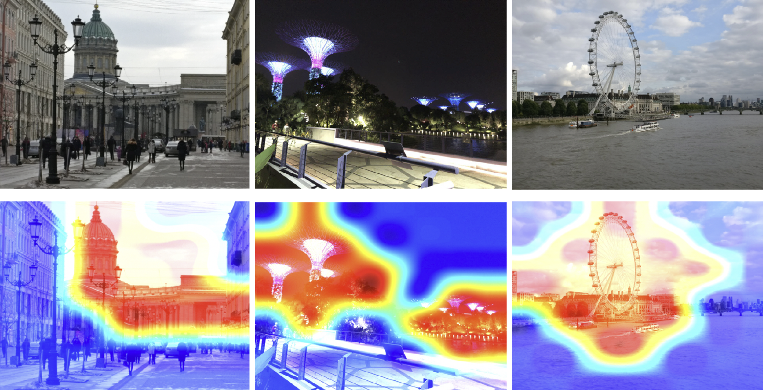
The heatmap shows which parts of the image the network pays more attention to. From the class activation map it can be seen that our neural network has successfully learned the concept of attraction.
Inference
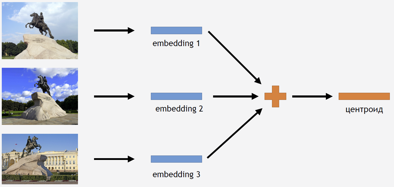
Now you need to somehow use this knowledge to get the result. Since we used Center loss for training, it seems quite logical at inference to also calculate tserotoid for attractions.
For this, we take part of the images from the training set for some kind of attraction, for example, for the Bronze Horseman. We run them through the network, get embeddings, average and get a centroid.
But the question arises: how many centroids for one attraction does it make sense to calculate? At first, the answer seems clear and logical: one centroid. But this turned out to be not quite so. At first, we also decided to make one centroid and got a pretty good result. So why do you need to take a few centroids?
Firstly, our data is not entirely clean. Although we cleaned the dataset, we removed only outright garbage. And we could have images that could not be considered garbage, but which worsen the result.
For example, I have a Winter Palace landmark class. I want to count a centroid for him. But the set included a number of photographs with Palace Square and the arch of the General Staff Building. If we consider the centroid in all images, it will turn out not too stable. It is necessary to somehow cluster their embeddings, which are obtained from an ordinary grid, take only the centroid that is responsible for the Winter Palace, and calculate the average according to these data.
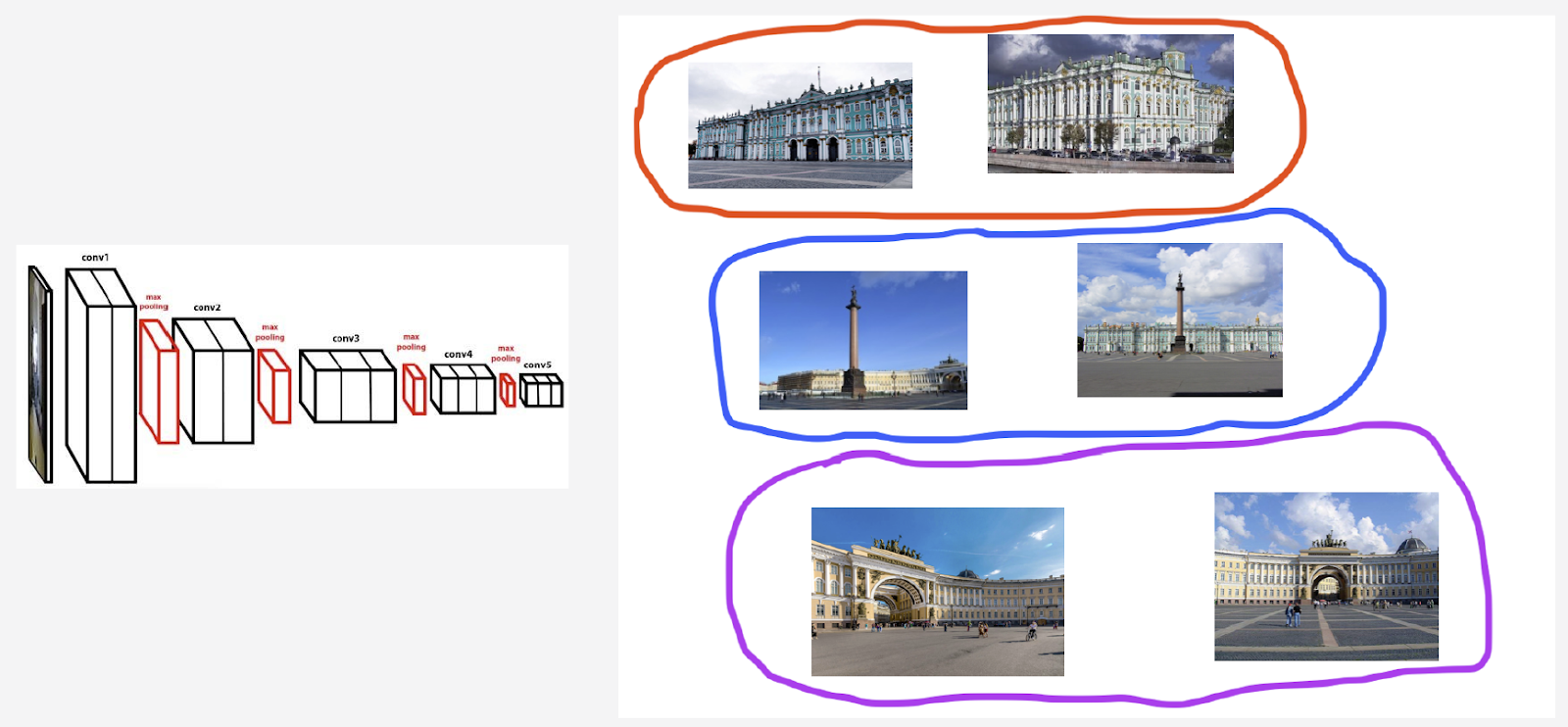
Secondly, photographs can be taken from different angles.
I will cite the Belfort bell tower in Bruges as an illustration of this behavior. Two centroids are counted for her. In the upper row of the image are those photos that are closer to the first centroid, and in the second row - those that are closer to the second centroid:

The first centroid is responsible for the more “ceremonial” close-up photos taken from the Bruges market square. And the second centroid is responsible for photographs taken from afar, from adjacent streets.
It turns out that by calculating several centroids per class of a point of interest, we can display different angles of this point of interest in inference.
So, how do we find these sets to calculate centroids? We apply hierarchical clustering to the datasets for each point of interest - complete link. With its help, we find valid clusters by which we will calculate centroids. By valid clusters we mean those that, as a result of clustering, contain at least 50 photographs. The remaining clusters are discarded. As a result, it turned out that about 20% of the sights have more than one centroid.
Now inference. We calculate it in two stages: first, we run the input image through our convolutional neural network and get embedding, and then using the scalar product we compare embedding with centroids. If the images contain geodata, then we restrict the search to centroids, which relate to the attractions located in a square of 1 per 1 km from the shooting location. This allows you to search more precisely, choose a lower threshold for subsequent comparison. If the obtained distance is greater than the threshold, which is a parameter of the algorithm, then we say that in the photo there is a point of interest with the maximum value of the scalar product. If less, then this is not a tourist attraction.
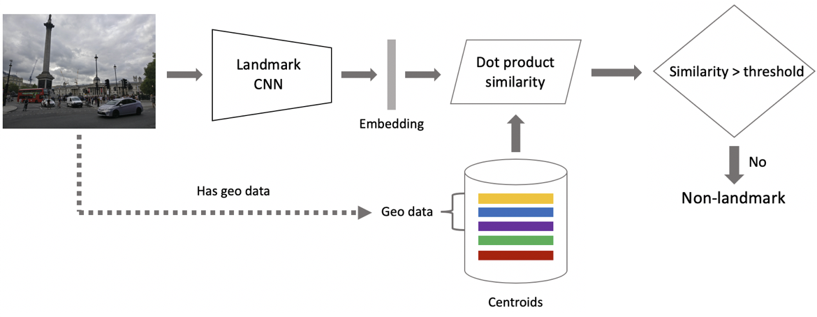
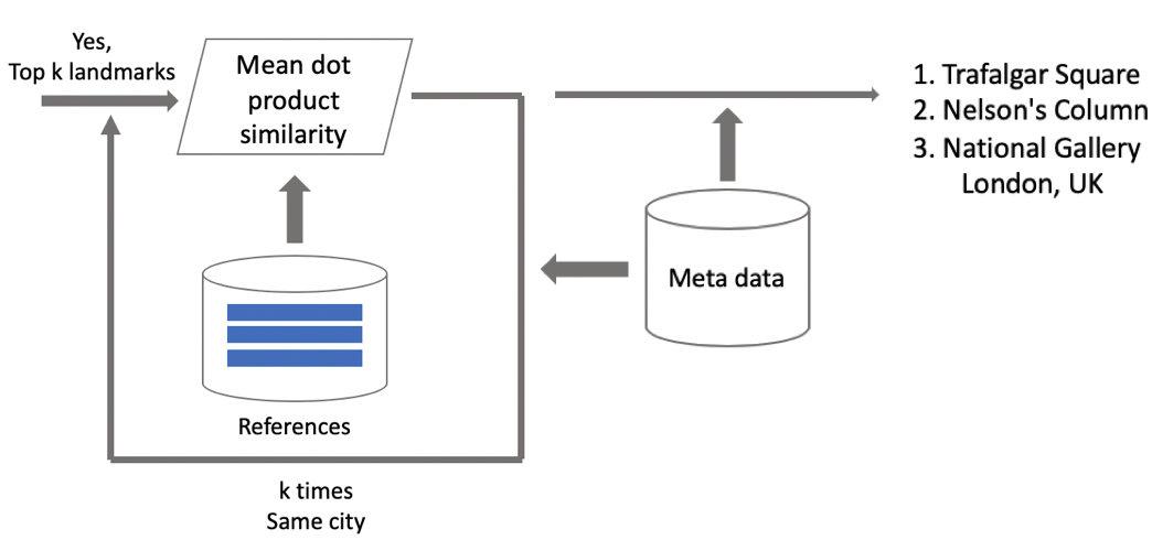
Suppose the photo contains a landmark. If we have geodata, then we use them and display the answer. If there is no geodata, then we do an additional check. When we cleaned the dataset, we made a set of reference images for each class of attractions. For them, we can count the embeddings, and then we calculate the average distance from them to the embedding of the request picture. If it is more than some threshold, then verification is passed, we include metadata and display the result. It is important to note that we can do such a procedure for several attractions that were found in the image.
Test results
We compared our model with DELF, for which we took the parameters at which it showed the best results on our test. The results were almost the same.
| Model | sights | No attractions |
|---|---|---|
| Our | 80% | 99% |
| Delf | 80.1% | 99% |
Then we divided the sights into two types: frequent (more than 100 photos), which make up 87% of all the sights in the test, and rare. Frequently, our model works well: accuracy of 85.3%. With rare sights, we got 46%, which is also very good - even with a small amount of data, our approach shows decent results.
| A type | Accuracy | Share of total |
|---|---|---|
| Frequent | 85.3% | 87% |
| Rare | 46% | thirteen % |
After we conducted A / B testing on user photos. As a result, the conversion of buying a place in the cloud increased by 10%, the conversion rate for removing a mobile application fell by 3%, and the number of views of albums increased by 13%.
Compare the speed of our approach and DELF. On a GPU, DELF requires 7 grid runs because it uses 7 image scales, and our approach uses only 1 run. On the CPU, DELF uses a longer search by the nearest neighbors method and a very long geometric verification. As a result, our method on the CPU was 15 times faster. In both cases, our approach wins in speed, which is extremely important during operation.
Results: holiday experience
At the beginning of the article, I mentioned the solution to the problem of scrolling and finding the right pictures with attractions. Here it is.
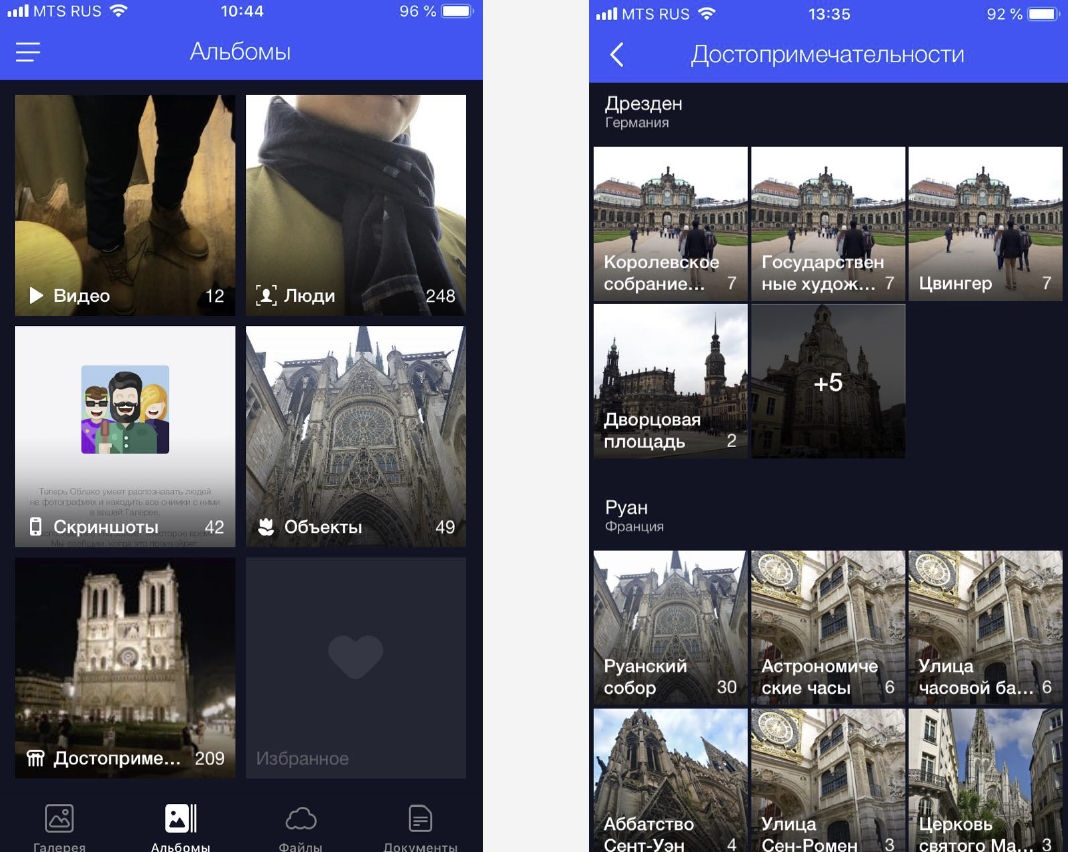
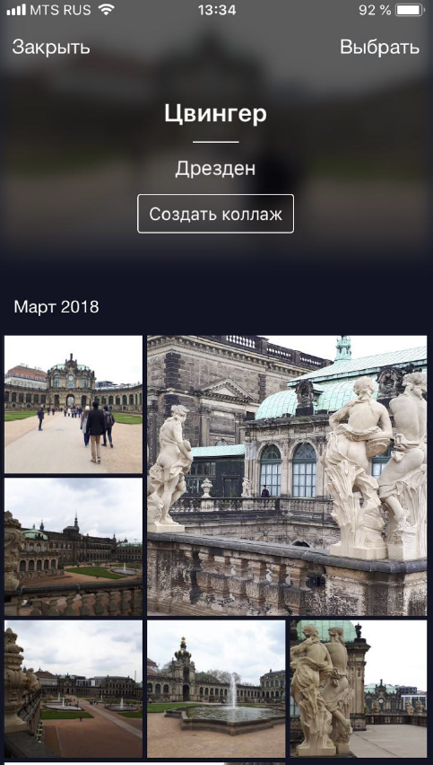
This is my cloud, and in it all the photos are divided into albums. There is an album "People", "Objects", "Sights". Inside it, the attractions are broken down by albums, which are grouped by city. If you click on the Zwinger in Dresden, then an album with photos of only this attraction will open.
A very useful feature: I went on vacation, took a picture, put it in a cloud. And when you wanted to upload them to Instagram or share with friends and relatives, you don’t have to search and choose for a long time, just a few clicks - and you will find the photos you need.
Summary
Let me remind you of the main points of our decision.
- Semi-automatic base cleaning. A bit of manual labor for the initial layout, and then the neural network copes itself. This allows you to quickly clean new data and train the model on it.
- We use deep convolutional neural networks and deep metric learning, which allows us to effectively learn the structure in classes.
- As a training paradigm, we used curriculum learning - learning in parts. This approach has helped us a lot. At inference, we use several centroids that allow you to use cleaner data and find different angles of attractions.
It would seem that object recognition is a well-studied area. But exploring the needs of real users, we find interesting new tasks, such as the recognition of attractions. It allows using machine learning to tell people something new about the world. It is very inspiring and motivating!