Speeding up data exploration using the pandas-profiling library
- Transfer
First of all, getting started with a new data set, you need to understand it. In order to do this, you need, for example, to find out the ranges of values accepted by the variables, their types, and also to find out about the number of missing values.
The pandas library provides us with many useful tools for performing Exploratory Data Analysis (EDA). But before using them, you usually need to start with more general functions, such as df.describe (). True, it should be noted that the possibilities provided by such functions are limited, and the initial stages of working with any data sets during EDA are very often very similar to each other.

The author of the material that we publish today says that he is not a fan of repeating actions. As a result, in search of tools to quickly and efficiently perform exploratory data analysis, he found the pandas-profiling library . The results of her work are expressed not in the form of certain individual indicators, but in the form of a rather detailed HTML report containing most of the information about the analyzed data that you may need to know before proceeding with more dense work with them.
Here we will consider the features of using the pandas-profiling library using the example of the Titanic dataset.
I decided to experiment with pandas-profiling on the Titanic dataset due to the fact that it has data of different types and because of the missing values in it. I believe that the pandas-profiling library is especially interesting in cases where the data has not yet been cleared and require further processing, depending on their features. In order to successfully perform such processing, you need to know where to start and what to look for. This is where pandas-profiling features come in handy.
To begin, we import the data and use pandas to obtain descriptive statistics indicators:
After executing this piece of code, you get what is shown in the following figure.
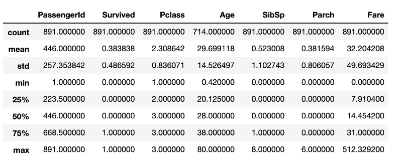
Indicators of descriptive statistics obtained using standard pandas tools
Although there is a lot of useful information here, there is not everything that would be interesting to learn about the data under study. For example, we can assume that in the data frame, in the structure
Now do the same using pandas-profiling:
The execution of the above line of code will allow you to generate a report with indicators of exploratory data analysis. The code shown above will lead to the conclusion of the found information about the data, but it can be done so that the result would be an HTML file, which, for example, can be shown to someone.
The first part of the report will contain the Overview section, which provides basic information about the data (number of observations, number of variables, and so on). In addition, it will contain a list of warnings that notify the analyst about what you should pay special attention to. These warnings can serve as a hint about where you can focus your efforts when clearing data.
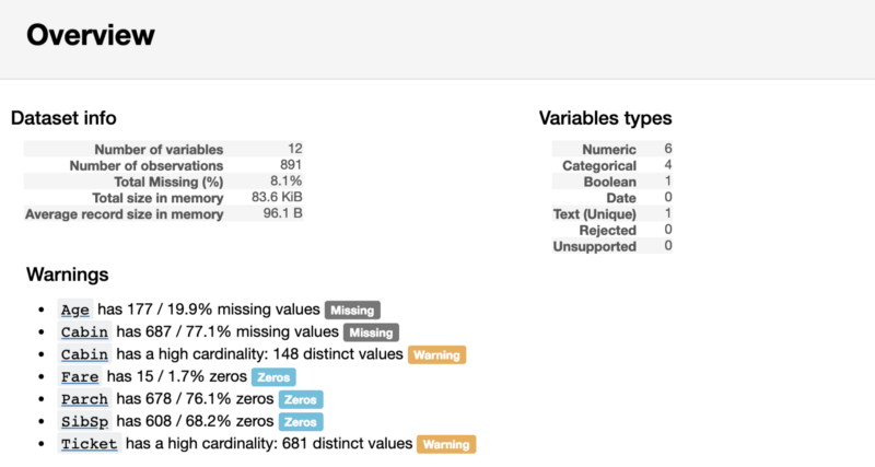
Report Section Overview
Behind the Overview section of the report, you can find useful information about each variable. Among other things, they include small charts that describe the distribution of each variable.

Information on the numerical variable Age
As you can see from the previous example, pandas-profiling gives us some useful indicators, such as the percentage and number of missing values, as well as indicators of descriptive statistics that we have already seen. Since
When considering a categorical variable, the displayed indicators are slightly different from those found for the numerical variable.

Information about the categorical variable Sex
Namely, instead of finding the average, minimum and maximum, the pandas-profiling library found the number of classes. Since it
If you, like me, like to research the code, then you may be interested in how exactly the pandas-profiling library calculates these indicators. Knowing this, given that the library code is open and available on GitHub, is not so difficult. Since I am not a big fan of using “black boxes” in my projects, I looked at the source code of the library. For example, here is the mechanism for processing numerical variables represented by the describe_numeric_1d function :
Although this piece of code may seem rather large and complex, in fact, it is very easy to understand. The point is that in the source code of the library there is a function that determines the types of variables. If it turned out that the library met a numerical variable, the above function will find the indicators that we considered. This function uses standard pandas operations for working with type objects
After the results of the analysis of variables, pandas-profiling, in the Correlations section, displays the Pearson and Spearman correlation matrices.
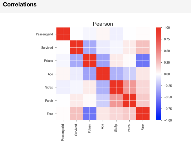
Pearson correlation matrix
If necessary, it is possible, in that line of code that starts the report generation, to set the threshold values used in calculating the correlation. By doing this, you can indicate what correlation strength is considered important for your analysis.
Finally, the pandas-profiling report, in the Sample section, displays, as an example, a piece of data taken from the beginning of the data set. This approach can lead to unpleasant surprises, since the first few observations can be a sample that does not reflect the characteristics of the entire data set.

The section containing the sample of the studied data
As a result, I do not recommend paying attention to this last section. Instead, it’s better to use a team
Summing up the foregoing, it can be noted that the pandas-profiling library provides the analyst with some useful features that come in handy in cases where you need to quickly get a general rough idea of the data or send someone a report on intelligence data analysis. At the same time, real work with data, taking into account their features, is performed, as without using pandas-profiling, manually.
If you want to take a look at what the whole intelligence analysis of data looks like in one Jupyter-notebook - take a look at this my project created using nbviewer. And in this GitHub repository you can find the appropriate code.
Dear readers! How do you start analyzing new data sets?

The pandas library provides us with many useful tools for performing Exploratory Data Analysis (EDA). But before using them, you usually need to start with more general functions, such as df.describe (). True, it should be noted that the possibilities provided by such functions are limited, and the initial stages of working with any data sets during EDA are very often very similar to each other.

The author of the material that we publish today says that he is not a fan of repeating actions. As a result, in search of tools to quickly and efficiently perform exploratory data analysis, he found the pandas-profiling library . The results of her work are expressed not in the form of certain individual indicators, but in the form of a rather detailed HTML report containing most of the information about the analyzed data that you may need to know before proceeding with more dense work with them.
Here we will consider the features of using the pandas-profiling library using the example of the Titanic dataset.
Pandas exploration data analysis
I decided to experiment with pandas-profiling on the Titanic dataset due to the fact that it has data of different types and because of the missing values in it. I believe that the pandas-profiling library is especially interesting in cases where the data has not yet been cleared and require further processing, depending on their features. In order to successfully perform such processing, you need to know where to start and what to look for. This is where pandas-profiling features come in handy.
To begin, we import the data and use pandas to obtain descriptive statistics indicators:
# импорт необходимых пакетов
import pandas as pd
import pandas_profiling
import numpy as np
# импорт данных
df = pd.read_csv('/Users/lukas/Downloads/titanic/train.csv')
# вычисление показателей описательной статистики
df.describe()
After executing this piece of code, you get what is shown in the following figure.

Indicators of descriptive statistics obtained using standard pandas tools
Although there is a lot of useful information here, there is not everything that would be interesting to learn about the data under study. For example, we can assume that in the data frame, in the structure
DataFrame, there are 891 rows. If you need to check this, you will need another line of code that determines the size of the frame. Although these calculations are not particularly resource intensive, their constant repetition will necessarily lead to loss of time, which is probably better spent on data cleaning.Exploration data analysis using pandas-profiling
Now do the same using pandas-profiling:
pandas_profiling.ProfileReport(df)The execution of the above line of code will allow you to generate a report with indicators of exploratory data analysis. The code shown above will lead to the conclusion of the found information about the data, but it can be done so that the result would be an HTML file, which, for example, can be shown to someone.
The first part of the report will contain the Overview section, which provides basic information about the data (number of observations, number of variables, and so on). In addition, it will contain a list of warnings that notify the analyst about what you should pay special attention to. These warnings can serve as a hint about where you can focus your efforts when clearing data.

Report Section Overview
Exploratory Variable Analysis
Behind the Overview section of the report, you can find useful information about each variable. Among other things, they include small charts that describe the distribution of each variable.

Information on the numerical variable Age
As you can see from the previous example, pandas-profiling gives us some useful indicators, such as the percentage and number of missing values, as well as indicators of descriptive statistics that we have already seen. Since
Agethis is a numerical variable, visualization of its distribution in the form of a histogram allows us to conclude that we have a right-angled distribution. When considering a categorical variable, the displayed indicators are slightly different from those found for the numerical variable.

Information about the categorical variable Sex
Namely, instead of finding the average, minimum and maximum, the pandas-profiling library found the number of classes. Since it
Sexis a binary variable, its values are represented by two classes. If you, like me, like to research the code, then you may be interested in how exactly the pandas-profiling library calculates these indicators. Knowing this, given that the library code is open and available on GitHub, is not so difficult. Since I am not a big fan of using “black boxes” in my projects, I looked at the source code of the library. For example, here is the mechanism for processing numerical variables represented by the describe_numeric_1d function :
def describe_numeric_1d(series, **kwargs):
    """Compute summary statistics of a numerical (`TYPE_NUM`) variable (a Series).
    Also create histograms (mini an full) of its distribution.
    Parameters
    ----------
    series : Series
        The variable to describe.
    Returns
    -------
    Series
        The description of the variable as a Series with index being stats keys.
    """
    # Format a number as a percentage. For example 0.25 will be turned to 25%.
    _percentile_format = "{:.0%}"
    stats = dict()
    stats['type'] = base.TYPE_NUM
    stats['mean'] = series.mean()
    stats['std'] = series.std()
    stats['variance'] = series.var()
    stats['min'] = series.min()
    stats['max'] = series.max()
    stats['range'] = stats['max'] - stats['min']
    # To avoid to compute it several times
    _series_no_na = series.dropna()
    for percentile in np.array([0.05, 0.25, 0.5, 0.75, 0.95]):
        # The dropna() is a workaround for https://github.com/pydata/pandas/issues/13098
        stats[_percentile_format.format(percentile)] = _series_no_na.quantile(percentile)
    stats['iqr'] = stats['75%'] - stats['25%']
    stats['kurtosis'] = series.kurt()
    stats['skewness'] = series.skew()
    stats['sum'] = series.sum()
    stats['mad'] = series.mad()
    stats['cv'] = stats['std'] / stats['mean'] if stats['mean'] else np.NaN
    stats['n_zeros'] = (len(series) - np.count_nonzero(series))
    stats['p_zeros'] = stats['n_zeros'] * 1.0 / len(series)
    # Histograms
    stats['histogram'] = histogram(series, **kwargs)
    stats['mini_histogram'] = mini_histogram(series, **kwargs)
    return pd.Series(stats, name=series.name)
Although this piece of code may seem rather large and complex, in fact, it is very easy to understand. The point is that in the source code of the library there is a function that determines the types of variables. If it turned out that the library met a numerical variable, the above function will find the indicators that we considered. This function uses standard pandas operations for working with type objects
Series, like series.mean(). The calculation results are stored in the dictionary stats. Histograms are formed using an adapted version of the function matplotlib.pyplot.hist. Adaptation aims to enable the function to work with various types of data sets.Correlation indicators and sample of the studied data
After the results of the analysis of variables, pandas-profiling, in the Correlations section, displays the Pearson and Spearman correlation matrices.

Pearson correlation matrix
If necessary, it is possible, in that line of code that starts the report generation, to set the threshold values used in calculating the correlation. By doing this, you can indicate what correlation strength is considered important for your analysis.
Finally, the pandas-profiling report, in the Sample section, displays, as an example, a piece of data taken from the beginning of the data set. This approach can lead to unpleasant surprises, since the first few observations can be a sample that does not reflect the characteristics of the entire data set.

The section containing the sample of the studied data
As a result, I do not recommend paying attention to this last section. Instead, it’s better to use a team
df.sample(5)that randomly selects 5 cases from the data set.Summary
Summing up the foregoing, it can be noted that the pandas-profiling library provides the analyst with some useful features that come in handy in cases where you need to quickly get a general rough idea of the data or send someone a report on intelligence data analysis. At the same time, real work with data, taking into account their features, is performed, as without using pandas-profiling, manually.
If you want to take a look at what the whole intelligence analysis of data looks like in one Jupyter-notebook - take a look at this my project created using nbviewer. And in this GitHub repository you can find the appropriate code.
Dear readers! How do you start analyzing new data sets?

