Deep Learning in Optical Flow Computation
With the advent of many different neural network architectures, many classic Computer Vision techniques are a thing of the past. Less and less often people use SIFT and HOG for object detection, and MBH for action recognition, and if they use it, it’s more like handcrafted signs for the corresponding grids. Today we are going to look at one of the classic CV problems in which the classical methods still hold the lead, while DL architectures languidly breathe them in the back of the head.
The task of computing the optical flow between two images (usually between adjacent frames of a video) is to construct a vector field the same size, moreover
  will correspond to the apparent pixel displacement vector
  from the first frame to the second. By constructing such a vector field between all adjacent frames of the video, we get a complete picture of how certain objects moved on it. In other words, this is the task of tracking all the pixels in a video. The optical flow is used extremely widely - in action recognition tasks, for example, such a vector field allows you to concentrate on the movements occurring on the video and get away from its context [7]. Even more common applications are visual odometry, video compression, post-processing (for example, adding a slow motion effect) and much more.
There is room for some ambiguities - what exactly is considered a visible bias from the point of view of mathematics? Usually, it is assumed that the pixel values go from one frame to the next without changes, in other words: - pixel intensity in coordinates then optical flow
  shows where this pixel has moved to the next point in time (i.e., on the next frame).
In the picture, it looks like this:
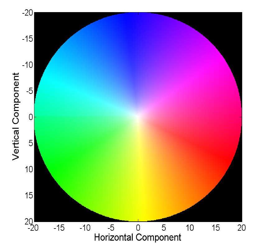
Visualizing a vector field directly with vectors is visual, but not always convenient, therefore the second common way is color visualization:


Each color in this picture encodes a specific vector. For simplicity, vectors longer than 20 are cropped, and the vector itself can be restored by color from the following image:
Classical methods have achieved pretty good accuracy, which sometimes comes at a price. We will consider the progress that neural networks have achieved in solving this problem over the past 4 years.
Two words about what datasets were available and popular at the beginning of our story (i.e., 2015), and how to measure the quality of the resulting algorithm.
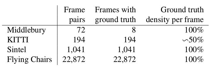
A tiny dataset of 8 pairs of images with small offsets, which, nevertheless, is sometimes used in validating algorithms for calculating the optical flux even now.

This is a dataset marked up for applications for self-driving cars and assembled using LIDAR technology. It is widely used to validate optical flow calculation algorithms and contains many rather complicated cases with sharp transitions between frames.

Another very common benchmark created on the basis of Sintel's open and drawn in Blender cartoon in two versions, which are designated as clean and final. The second is much more complicated, because contains a lot of atmospheric effects, noise, blur and other troubles for the algorithms for calculating the optical flux.
The standard error function for the optical flow computation task is End Point Error or EPE. This is simply the Euclidean distance between the calculated algorithm and the true optical flux, averaged over all pixels.
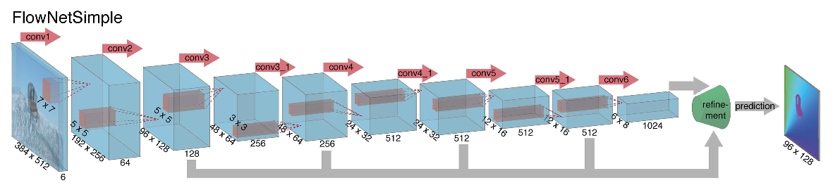
Взявшись за построение архитектуры нейронной сети для задачи вычисления оптического потока в далеком 2015, авторы (из Мюнхенского и Фрайбургского университетов) столкнулись с двумя проблемами: под данную задачу не было большого размеченного датасета, а его разметка вручную составляла бы определенные сложности (попробуй разметить куда двинулся каждый пиксель изображения на следующем кадре), во-первых. Данная задача довольно сильно отличалась от всех задач, которые решались при помощи CNN-архитектур до этого, во-вторых. По-сути, это задача попиксельной регрессии, что делает ее схожей с задачей сегментации (попиксельная классификация), но вместо одного изображения у нас на входе два, причем интуитивно, признаки должны каким-то образом показывать разницу между этими двумя изображениями. В качестве первой итерации было решено в качестве входа просто стакнуть два RGB-кадра (получив, по-сути, 6-канальное изображение), между которыми мы хотим подсчитать оптический поток, а в качестве архитектуры взять U-net с рядом изменений. Такую сеть назвали FlowNetS (S значит Simple):
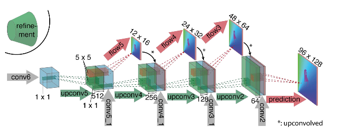
As you can see from the diagram, the encoder is not noticeable, the decoder differs from the classic options in several ways:
To understand how the authors tried to improve their base line, you need to know what the correlation between images is and why it can be useful in calculating the optical flux. So, having two images and knowing that the second is the next frame in the video relative to the first, we can try to compare the area around the point on the first frame (for which we want to find a shift to the second frame) with areas of the same size in the second image. Moreover, assuming that the shift could not be too large per unit time, the comparison can be considered only in a certain neighborhood of the starting point. For this, cross-correlation is used. Let us illustrate with an example.
Take two adjacent frames of the video, we want to determine where a certain point has shifted from the first frame to the second. Suppose that some area around this point has shifted in the same way. Indeed, neighboring pixels in a video are usually offset together, as most likely, visually, are part of one object. This assumption is actively used, for example, in differential approaches, which can be read in more detail in [5], [6].
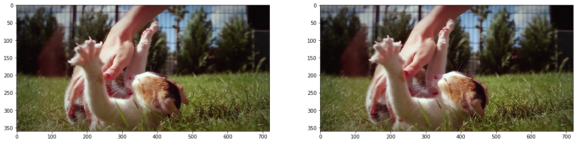
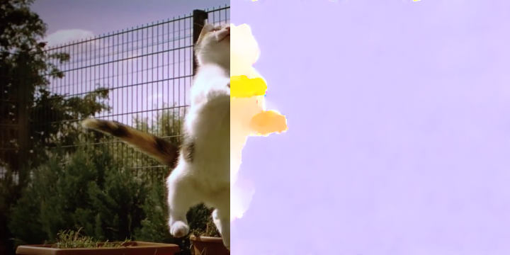
Let's try to take a point in the center of the kitten's paw and find it on the second frame. Take some area around it.
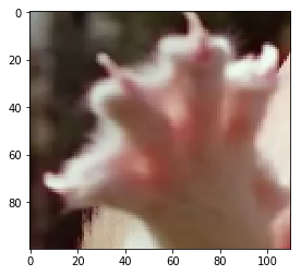
We calculate the correlation between this area (in English literature often write template or patch from the first image) and the second image. The template will simply “walk” through the second image and calculate the next value between itself and pieces of the same size in the second image:
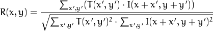
The larger the value of this value, the more the template looks like the corresponding piece in the second image. With OpenCV, this can be done like this:
More details can be found in [7].
The result is as follows:
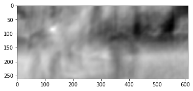
We see an explicit peak, indicated by white. Find it in the second frame:

We see that the foot was found correctly, according to these data we can understand in which direction it moved from the first frame to the second and calculate the corresponding optical flux. In addition, it turns out that this operation is quite resistant to photometric distortions, i.e. if the brightness in the second frame rises sharply, the cross-correlation peak between images will remain in place.
Considering all the above, the authors decided to introduce the so-called correlation layer into their architecture, but it was decided not to consider the correlation according to the input images, but according to the feature maps after several layers of the encoder. Such a layer, for obvious reasons, does not have learning parameters, although it is similar in essence to convolution, but instead of filters, here we use not weights, but some area of the second image:
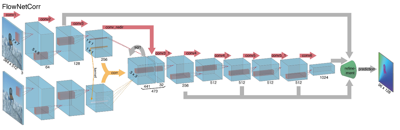
Oddly enough, this trick did not give a significant improvement in the quality of the authors of this article, however, it was more successfully applied in further works, and in [9] the authors were able to show that by slightly changing the training parameters, FlowNetC can be made to work much better.
The authors solved the problem with the lack of a dataset in a rather elegant way: they scraped 964 images from Flickr on the themes: "city", "landscape", "mountain" in the resolution of 1024 × 768 and used their crop 512 × 384 as a background, which then threw a few chairs from an open set of rendered 3D models. Then, various affine transformations were independently applied to the chairs and the background, which were used to generate the second image in a pair and the optical flow between them. The result is as follows:

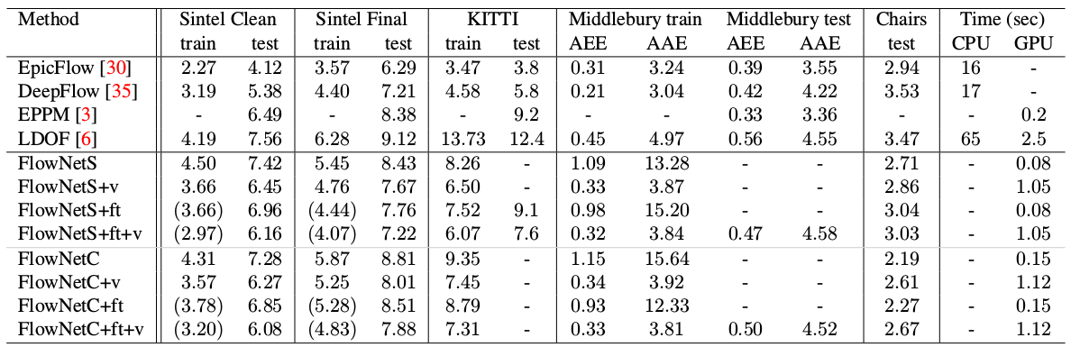
An interesting result was that the use of such a synthetic dataset made it possible to achieve relatively good quality for data from another domain. The fine tun on the corresponding data, of course, proved more qualities (+ ft in the table below):
The result on real videos can be seen here:
In many subsequent articles, the authors tried to improve quality by solving the problem of poor recognition of sudden movements. Intuitively, the movement will not be captured by the network if its vector significantly goes beyond the receptive field of activation. It is proposed to solve this problem due to three things: a larger convolution, pyramids and “warping” one image from a pair into an optical stream. Everything in order.
So, if we have a couple of images in which the object has sharply shifted (10+ pixels), then we can simply reduce the image (by 6 or more times). The absolute value of the offset will decrease significantly, and the network is more likely to be able to “catch” it, especially if its convolutions are larger than the offset itself (in this case, 7x7 convolutions are used).
However, when reducing the image, we lost a lot of important details, so we should go to the next level of the pyramid, in which the image size is already larger, while somehow taking into account the information that we received before when we calculated the optical flux at a smaller size. This is done using the warping operator, which recounts the first image according to the available approximation of the optical flux (obtained at the previous level). An improvement in this case is that the first image that is “pushed” according to the approximation of the optical flux will be closer to the second than the original one, that is, we again reduce the absolute value of the optical flux, which we need to predict (recall, small in value movements are detected much better, since they are completely included in one convolution). In terms of mathematics, , i.e. a specific point in the image
 - the image itself
  - optical flow
  - the resulting image, "wrapped" in the optical stream.
How to apply all this in CNN architecture? We fix the number of pyramid levels and a factor by which each subsequent image is reduced at a level starting from the last
  . Denote by
 and
and  the downsampling and upsampling functions of the image or optical flux by this factor.
We’ll also get a set of CNN-ok { }, one for each level of the pyramid. Then
 -th network will accept a couple of images with
  pyramid level and optical flux calculated on
  level (
 will just accept a tensor of zeros instead). In this case, we will send one of the images to the warping layer to reduce the difference between them, and we will not predict the optical flux at this level, but the value that needs to be added to the increased (upsampled) optical flux from the previous level to obtain the optical flux at this level. In the formula, it looks something like this:
To get the optical stream itself, we simply add the network predicate and the increased stream from the previous level:

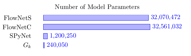
The advantage of this approach is that we can teach each level independently. The authors began training from level 0, each subsequent network was initialized with the parameters of the previous one. Since every networksolves the problem much simpler than the full calculation of the optical flux in a large image, then the parameters can be made much less. So much so that now the whole ensemble can fit on mobile devices:
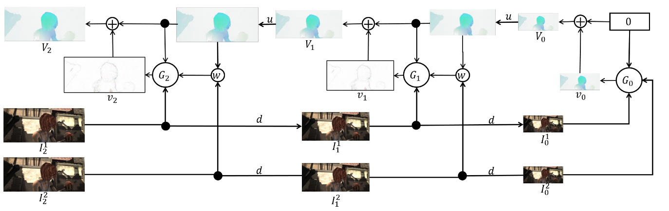
The ensemble itself looks like this (an example of a pyramid of 3 levels): It
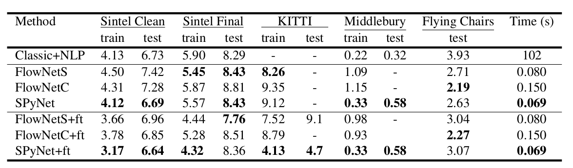
remains to talk directly about architecturenetwork and take stock. Every networkconsists of 5 convolutional layers, each of which ends with ReLU activation, except for the last (which predicts the optical flow). The number of filters on each layer is respectively { }. The inputs of the neural network (the image, the second image “wrapped” in the optical stream and the optical stream itself) simply concatenate according to the dimension of the channels, so their input tensor has 8. The results are impressive:
Inspired by the success of their German colleagues, the guys from NVIDIA decided to apply their experience (and video cards) to further improve the result. Their work was largely based on ideas from the previous model (SpyNet), so PWC-Net will also deal with pyramids, but with convolution pyramids, not the original images, however, again - in order.
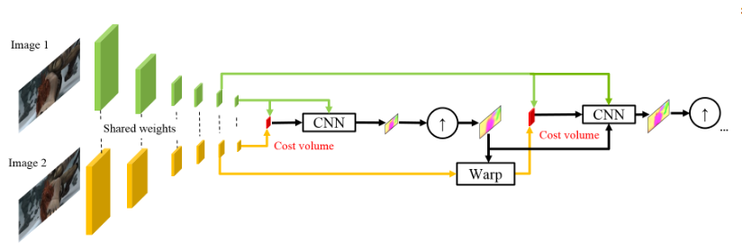
Using raw pixel intensities to calculate the optical flux is not always reasonable, because A sharp change in brightness / contrast will break our assumption that pixels move from one frame to the next without changes and the algorithm will not be resistant to such changes. In classical algorithms for calculating the optical flux, various transformations are used that mitigate this situation, in this case, the authors decided to provide the model with the opportunity to learn such transformations themselves. Therefore, instead of the image pyramid in PWC-Net, convolution pyramids are used (hence the first letter in Pwc-Net), i.e. just feature maps from different CNN layers, which is called feature pyramid extractor here.
Then everything is almost like in SpyNet, just before you submit to CNN, which is called optical flow estimator, everything you need, namely:
between the “wrapped” second frame and the usual first (again I remind you that instead of raw images, feature cards with feature pyramid extractor are used here) consider what is called cost volume (hence the third letter in pwC-Net) and which is essentially already previously considered correlation between two images.
The final touch is the context network, which is added immediately after the optical flow estimator and plays the role of trained post-processing for the calculated optical stream. Architectural details can be viewed under the spoiler or in the original article.
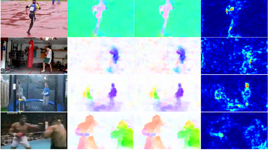
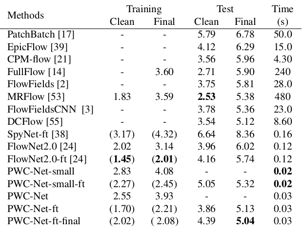
The results are even more impressive:
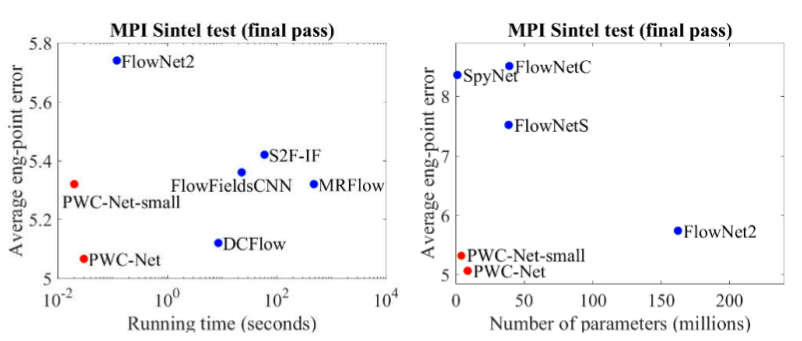
Compared to other CNN methods for calculating optical flow, PWC-Net achieves a balance between quality and quantity of parameters:
There is also an excellent presentation by the authors themselves, in which they talk about the model itself and their experiments:
The evolution of architectures that solve the problem of optical flux counting is a wonderful example of how progress in CNN architectures and combining them with classical methods gives the best and best result. And while classic CV methods still win in quality, recent results give hope that this is fixable ...
1. FlowNet: Learning Optical Flow with Convolutional Networks: article , code .
2. Large displacement optical flow: descriptor matching in variational motion estimation: article .
3. Optical Flow Estimation using a Spatial Pyramid Network: article , code .
4. PWC-Net: CNNs for Optical Flow Using Pyramid, Warping, and Cost Volume: article , code .
5. What you wanted to know about the optical flow, but were embarrassed to ask: article .
6. Calculation of the optical flux by the Lucas-Canada method. Theory: article .
7. Template matching with OpenCVP:дока.
8. Quo Vadis, Action Recognition? A New Model and the Kinetics Dataset: статья.
9. FlowNet 2.0: Evolution of Optical Flow Estimation with Deep Networks: статья, код.
Optical flow estimation
The task of computing the optical flow between two images (usually between adjacent frames of a video) is to construct a vector field
the same size, moreover will correspond to the apparent pixel displacement vector from the first frame to the second. By constructing such a vector field between all adjacent frames of the video, we get a complete picture of how certain objects moved on it. In other words, this is the task of tracking all the pixels in a video. The optical flow is used extremely widely - in action recognition tasks, for example, such a vector field allows you to concentrate on the movements occurring on the video and get away from its context [7]. Even more common applications are visual odometry, video compression, post-processing (for example, adding a slow motion effect) and much more. There is room for some ambiguities - what exactly is considered a visible bias from the point of view of mathematics? Usually, it is assumed that the pixel values go from one frame to the next without changes, in other words:

- pixel intensity in coordinates then optical flow shows where this pixel has moved to the next point in time (i.e., on the next frame). In the picture, it looks like this:
Visualizing a vector field directly with vectors is visual, but not always convenient, therefore the second common way is color visualization:
Each color in this picture encodes a specific vector. For simplicity, vectors longer than 20 are cropped, and the vector itself can be restored by color from the following image:
More cat flow!


Classical methods have achieved pretty good accuracy, which sometimes comes at a price. We will consider the progress that neural networks have achieved in solving this problem over the past 4 years.
Data and Metrics
Two words about what datasets were available and popular at the beginning of our story (i.e., 2015), and how to measure the quality of the resulting algorithm.
Middlebury
A tiny dataset of 8 pairs of images with small offsets, which, nevertheless, is sometimes used in validating algorithms for calculating the optical flux even now.
Kitty
This is a dataset marked up for applications for self-driving cars and assembled using LIDAR technology. It is widely used to validate optical flow calculation algorithms and contains many rather complicated cases with sharp transitions between frames.
Sintel
Another very common benchmark created on the basis of Sintel's open and drawn in Blender cartoon in two versions, which are designated as clean and final. The second is much more complicated, because contains a lot of atmospheric effects, noise, blur and other troubles for the algorithms for calculating the optical flux.
EPE
The standard error function for the optical flow computation task is End Point Error or EPE. This is simply the Euclidean distance between the calculated algorithm and the true optical flux, averaged over all pixels.
Flownet (2015)
Взявшись за построение архитектуры нейронной сети для задачи вычисления оптического потока в далеком 2015, авторы (из Мюнхенского и Фрайбургского университетов) столкнулись с двумя проблемами: под данную задачу не было большого размеченного датасета, а его разметка вручную составляла бы определенные сложности (попробуй разметить куда двинулся каждый пиксель изображения на следующем кадре), во-первых. Данная задача довольно сильно отличалась от всех задач, которые решались при помощи CNN-архитектур до этого, во-вторых. По-сути, это задача попиксельной регрессии, что делает ее схожей с задачей сегментации (попиксельная классификация), но вместо одного изображения у нас на входе два, причем интуитивно, признаки должны каким-то образом показывать разницу между этими двумя изображениями. В качестве первой итерации было решено в качестве входа просто стакнуть два RGB-кадра (получив, по-сути, 6-канальное изображение), между которыми мы хотим подсчитать оптический поток, а в качестве архитектуры взять U-net с рядом изменений. Такую сеть назвали FlowNetS (S значит Simple):
As you can see from the diagram, the encoder is not noticeable, the decoder differs from the classic options in several ways:
- The prediction of the optical flow occurs not only from the last level, but also from all the others. To get Ground Truth for the i-th level of the decoder, the original target (i.e. the optical stream) is simply reduced (almost the same as the image) to the desired resolution, and the predicate obtained at the i-th level goes further, t i.e., it is concatenated with a feature map emerging from this level. The general function of training losses will be a weighted sum of losses from all levels of the decoder, while the weight itself will be the greater, the closer the level to the network output. The authors do not give an explanation of why this is done, but most likely the reason is the fact that sharp movements are better to detect at early levels, then the vectors in the lower-resolution optical stream will not be so large.
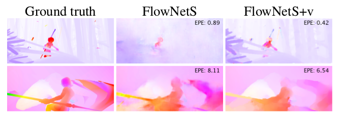
- The diagram shows that the input resolution of the images is 384x512, and the output is four times smaller. The authors noticed that if you increase this output to 384x512 by simple bilinear interpolation, it will give the same quality as if you attach two more levels of the decoder. You can also use the variational approach [2], which proves the quality (+ v in the table with quality).
- As in U-net, attribute cards from the encoder are sent to the decoder and concatenated as shown in the diagram.
To understand how the authors tried to improve their base line, you need to know what the correlation between images is and why it can be useful in calculating the optical flux. So, having two images and knowing that the second is the next frame in the video relative to the first, we can try to compare the area around the point on the first frame (for which we want to find a shift to the second frame) with areas of the same size in the second image. Moreover, assuming that the shift could not be too large per unit time, the comparison can be considered only in a certain neighborhood of the starting point. For this, cross-correlation is used. Let us illustrate with an example.
Take two adjacent frames of the video, we want to determine where a certain point has shifted from the first frame to the second. Suppose that some area around this point has shifted in the same way. Indeed, neighboring pixels in a video are usually offset together, as most likely, visually, are part of one object. This assumption is actively used, for example, in differential approaches, which can be read in more detail in [5], [6].
fig, ax = plt.subplots(1, 2, figsize=(20, 10))
ax[0].imshow(frame1)
ax[1].imshow(frame2);
Let's try to take a point in the center of the kitten's paw and find it on the second frame. Take some area around it.
patch1 = frame1[90:190, 140:250]
plt.imshow(patch1);
We calculate the correlation between this area (in English literature often write template or patch from the first image) and the second image. The template will simply “walk” through the second image and calculate the next value between itself and pieces of the same size in the second image:
The larger the value of this value, the more the template looks like the corresponding piece in the second image. With OpenCV, this can be done like this:
corr = cv2.matchTemplate(frame2, patch1, cv2.TM_CCORR_NORMED)
plt.imshow(corr, cmap='gray');
More details can be found in [7].
The result is as follows:
We see an explicit peak, indicated by white. Find it in the second frame:
min_val, max_val, min_loc, max_loc = cv2.minMaxLoc(corr)
h, w, _ = patch1.shape
top_left = max_loc
bottom_right = (top_left[0] + w, top_left[1] + h)
frame2_copy = frame2.copy()
cv2.rectangle(frame2_copy, top_left, bottom_right, 255, 2)
plt.imshow(frame2_copy);
We see that the foot was found correctly, according to these data we can understand in which direction it moved from the first frame to the second and calculate the corresponding optical flux. In addition, it turns out that this operation is quite resistant to photometric distortions, i.e. if the brightness in the second frame rises sharply, the cross-correlation peak between images will remain in place.
Considering all the above, the authors decided to introduce the so-called correlation layer into their architecture, but it was decided not to consider the correlation according to the input images, but according to the feature maps after several layers of the encoder. Such a layer, for obvious reasons, does not have learning parameters, although it is similar in essence to convolution, but instead of filters, here we use not weights, but some area of the second image:
Oddly enough, this trick did not give a significant improvement in the quality of the authors of this article, however, it was more successfully applied in further works, and in [9] the authors were able to show that by slightly changing the training parameters, FlowNetC can be made to work much better.
The authors solved the problem with the lack of a dataset in a rather elegant way: they scraped 964 images from Flickr on the themes: "city", "landscape", "mountain" in the resolution of 1024 × 768 and used their crop 512 × 384 as a background, which then threw a few chairs from an open set of rendered 3D models. Then, various affine transformations were independently applied to the chairs and the background, which were used to generate the second image in a pair and the optical flow between them. The result is as follows:
An interesting result was that the use of such a synthetic dataset made it possible to achieve relatively good quality for data from another domain. The fine tun on the corresponding data, of course, proved more qualities (+ ft in the table below):
The result on real videos can be seen here:
SpyNet (2016)
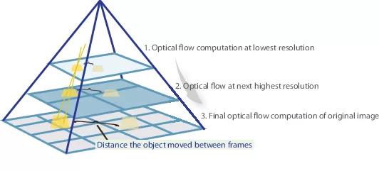
In many subsequent articles, the authors tried to improve quality by solving the problem of poor recognition of sudden movements. Intuitively, the movement will not be captured by the network if its vector significantly goes beyond the receptive field of activation. It is proposed to solve this problem due to three things: a larger convolution, pyramids and “warping” one image from a pair into an optical stream. Everything in order.
So, if we have a couple of images in which the object has sharply shifted (10+ pixels), then we can simply reduce the image (by 6 or more times). The absolute value of the offset will decrease significantly, and the network is more likely to be able to “catch” it, especially if its convolutions are larger than the offset itself (in this case, 7x7 convolutions are used).
However, when reducing the image, we lost a lot of important details, so we should go to the next level of the pyramid, in which the image size is already larger, while somehow taking into account the information that we received before when we calculated the optical flux at a smaller size. This is done using the warping operator, which recounts the first image according to the available approximation of the optical flux (obtained at the previous level). An improvement in this case is that the first image that is “pushed” according to the approximation of the optical flux will be closer to the second than the original one, that is, we again reduce the absolute value of the optical flux, which we need to predict (recall, small in value movements are detected much better, since they are completely included in one convolution). In terms of mathematics,

, i.e. a specific point in the image - the image itself - optical flow - the resulting image, "wrapped" in the optical stream. How to apply all this in CNN architecture? We fix the number of pyramid levels
and a factor by which each subsequent image is reduced at a level starting from the last . Denote by and the downsampling and upsampling functions of the image or optical flux by this factor. We’ll also get a set of CNN-ok {
}, one for each level of the pyramid. Then-th network will accept a couple of images with pyramid level and optical flux calculated on level (will just accept a tensor of zeros instead). In this case, we will send one of the images to the warping layer to reduce the difference between them, and we will not predict the optical flux at this level, but the value that needs to be added to the increased (upsampled) optical flux from the previous level to obtain the optical flux at this level. In the formula, it looks something like this:
To get the optical stream itself, we simply add the network predicate and the increased stream from the previous level:

The advantage of this approach is that we can teach each level independently. The authors began training from level 0, each subsequent network was initialized with the parameters of the previous one. Since every network
solves the problem much simpler than the full calculation of the optical flux in a large image, then the parameters can be made much less. So much so that now the whole ensemble can fit on mobile devices: The ensemble itself looks like this (an example of a pyramid of 3 levels): It
remains to talk directly about architecture
network and take stock. Every networkconsists of 5 convolutional layers, each of which ends with ReLU activation, except for the last (which predicts the optical flow). The number of filters on each layer is respectively {}. The inputs of the neural network (the image, the second image “wrapped” in the optical stream and the optical stream itself) simply concatenate according to the dimension of the channels, so their input tensor has 8. The results are impressive:PWC-Net (2018)
Inspired by the success of their German colleagues, the guys from NVIDIA decided to apply their experience (and video cards) to further improve the result. Their work was largely based on ideas from the previous model (SpyNet), so PWC-Net will also deal with pyramids, but with convolution pyramids, not the original images, however, again - in order.
Using raw pixel intensities to calculate the optical flux is not always reasonable, because A sharp change in brightness / contrast will break our assumption that pixels move from one frame to the next without changes and the algorithm will not be resistant to such changes. In classical algorithms for calculating the optical flux, various transformations are used that mitigate this situation, in this case, the authors decided to provide the model with the opportunity to learn such transformations themselves. Therefore, instead of the image pyramid in PWC-Net, convolution pyramids are used (hence the first letter in Pwc-Net), i.e. just feature maps from different CNN layers, which is called feature pyramid extractor here.
Then everything is almost like in SpyNet, just before you submit to CNN, which is called optical flow estimator, everything you need, namely:
- image (in this case, a feature map from feature pyramid extractor),
- the up-sampled optical flux calculated at the previous level,
- the second image, “wrapped” (remember the warping layer, hence the second letter in pWc-Net) into this optical stream,
between the “wrapped” second frame and the usual first (again I remind you that instead of raw images, feature cards with feature pyramid extractor are used here) consider what is called cost volume (hence the third letter in pwC-Net) and which is essentially already previously considered correlation between two images.
The final touch is the context network, which is added immediately after the optical flow estimator and plays the role of trained post-processing for the calculated optical stream. Architectural details can be viewed under the spoiler or in the original article.
Intimate details
Итак, feature pyramid extractor имеет одни и те же веса для обоих изображений, в качестве нелинейности для каждой свертки используется leaky ReLU. Для уменьшения разрешения карт признаков на каждом последующем уровне используются свертки со страйдом 2, а  означает карту признаков изображения
  на уровне
  .
.

Optical flow estimator на 2м уровне пирамиды (для примера). Здесь ничего необычного, каждая свертка по-прежнему заканчивается leaky ReLU, кроме последней, которая и предсказывает оптический поток.

Context network все на том же 2м уровне пирамиды, эта сеть использует dilated convolutions с теми же leaky ReLU активациями, кроме последнего слоя. Она принимает на вход вычисленный с помощью optical flow estimator оптический поток и признаки со второго с конца слоя с того же optical flow estimator. Последняя цифра в каждом блоке означает dilation constant.

означает карту признаков изображения на уровне .Optical flow estimator на 2м уровне пирамиды (для примера). Здесь ничего необычного, каждая свертка по-прежнему заканчивается leaky ReLU, кроме последней, которая и предсказывает оптический поток.
Context network все на том же 2м уровне пирамиды, эта сеть использует dilated convolutions с теми же leaky ReLU активациями, кроме последнего слоя. Она принимает на вход вычисленный с помощью optical flow estimator оптический поток и признаки со второго с конца слоя с того же optical flow estimator. Последняя цифра в каждом блоке означает dilation constant.
The results are even more impressive:
Compared to other CNN methods for calculating optical flow, PWC-Net achieves a balance between quality and quantity of parameters:
There is also an excellent presentation by the authors themselves, in which they talk about the model itself and their experiments:
Conclusion
The evolution of architectures that solve the problem of optical flux counting is a wonderful example of how progress in CNN architectures and combining them with classical methods gives the best and best result. And while classic CV methods still win in quality, recent results give hope that this is fixable ...
Sources and links
1. FlowNet: Learning Optical Flow with Convolutional Networks: article , code .
2. Large displacement optical flow: descriptor matching in variational motion estimation: article .
3. Optical Flow Estimation using a Spatial Pyramid Network: article , code .
4. PWC-Net: CNNs for Optical Flow Using Pyramid, Warping, and Cost Volume: article , code .
5. What you wanted to know about the optical flow, but were embarrassed to ask: article .
6. Calculation of the optical flux by the Lucas-Canada method. Theory: article .
7. Template matching with OpenCVP:дока.
8. Quo Vadis, Action Recognition? A New Model and the Kinetics Dataset: статья.
9. FlowNet 2.0: Evolution of Optical Flow Estimation with Deep Networks: статья, код.