Machine learning without Python, Anaconda and other reptiles
No, well, of course, I'm not serious. There must be a limit to what extent it is possible to simplify the subject. But for the first stages, an understanding of the basic concepts and a quick "entry" into the topic, it may be permissible. And how to properly name this material (options: “Machine learning for dummies”, “Analysis of data from the diapers”, “Algorithms for the smallest”), we will discuss at the end.
To business. He wrote several application programs on MS Excel for visualization and visualization of processes that occur in different machine learning methods when analyzing data. Seeing is believing, in the end, according to the media of the culture that developed most of these methods (by the way, by no means all. The most powerful “support vector method”, or SVM, support vector machine is an invention of our compatriot Vladimir Vapnik, Moscow Institute of Management. 1963, by the way! Now he, however, teaches and works in the USA).
Three files for review
Tasks of this kind relate to “learning without a teacher”, when we need to break down the initial data into a certain number of categories known in advance, but we don’t have any number of “correct answers”, we must extract them from the data itself. The fundamental classical problem of finding subspecies of iris flowers (Ronald Fisher, 1936!), Which is considered the first sign of this field of knowledge - is of such a nature.
The method is quite simple. We have a set of objects represented as vectors (sets of N numbers). For irises, these are sets of 4 numbers characterizing a flower: the length and width of the outer and inner perianth lobes, respectively ( Iris Fisher - Wikipedia ). As a distance, or measure of proximity between objects, the usual Cartesian metric is chosen.
Further, the centers of the clusters are selected arbitrarily (or not arbitrarily, see below), and the distances from each object to the centers of the clusters are calculated. Each object in this iteration step is marked as belonging to the nearest center. Then the center of each cluster is transferred to the arithmetic mean of the coordinates of its members (by analogy with physics it is also called the "center of mass"), and the procedure is repeated.
The process converges quickly enough. In the two-dimensional pictures, it looks like this:
1. The initial random distribution of points on the plane and the number of clusters

2. Setting the center of the clusters and assigning points to their clusters
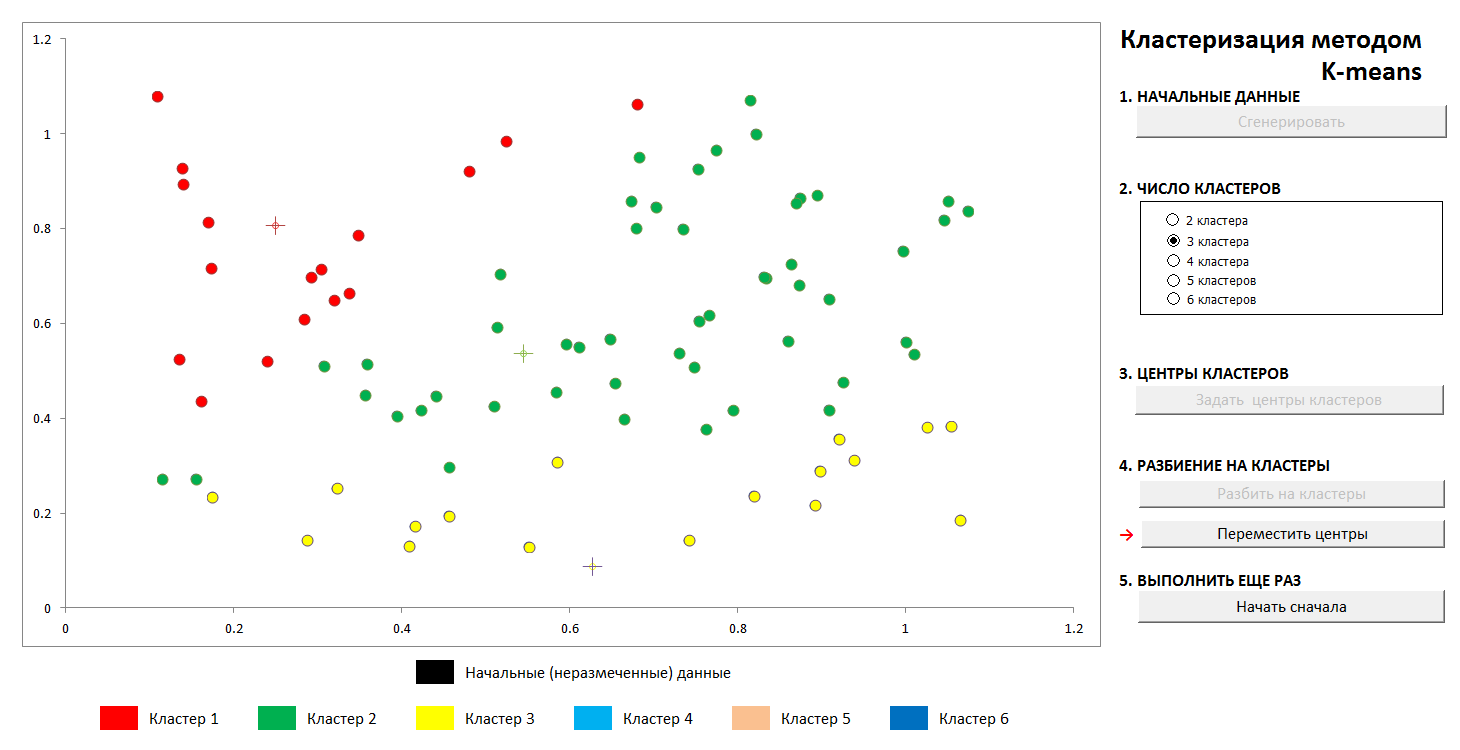
3. Transfer of coordinates of the centers of clusters, recalculation of the points, until the centers are stabilized. The trajectory of the center of the cluster to the final position is visible.

At any time, you can set new cluster centers (without generating a new distribution of points!) And see that the partitioning process is not always unique. Mathematically, this means that for the optimized function (the sum of the squares of the distances from the points to the centers of its clusters) we find not a global, but a local minimum. This problem can be defeated either by a non-random choice of the initial centers of the clusters, or by sorting out the possible centers (sometimes it is advantageous to place them exactly at some point, then at least there is a guarantee that we will not get empty clusters). In any case, a finite set always has an exact lower bound.
You can play with this file at this link (do not forget to enable macro support. Files have been checked for viruses)
Method description on Wikipedia - k-means method
A remarkable scientist and popularizer of data science K.V. Vorontsov briefly talks about machine learning methods as "the science of drawing curves through points." In this example, we will find the pattern in the data by the least squares method.
The technique of dividing the source data into “training” and “control”, as well as such a phenomenon as retraining, or “retraining” for the data is shown. With the correct approximation, we will have a certain error on the training data and a slightly larger error on the control data. If it’s wrong, it’s an exact adjustment to the training data and a huge mistake on the control.
(It is a well-known fact that through N points it is possible to draw a single curve of the N-1st degree, and this method generally does not give the desired result. The Lagrange interpolation polynomial on Wikipedia )
1. We set the initial distribution

2. Divide the points into “training” and “control” in the ratio of 70 to 30.

3. Draw an approximating curve by the training points, we see the error that it gives on the control data

4. Draw the exact curve through the training points, and we see a monstrous error on the control data (and zero on the training, but what's the point?).

Of course, the simplest variant with a single partition into “training” and “control” subsets is shown, in the general case this is done repeatedly for the best adjustment of the coefficients.
The file is available here, anti-virus checked. Turn on macros to work correctly
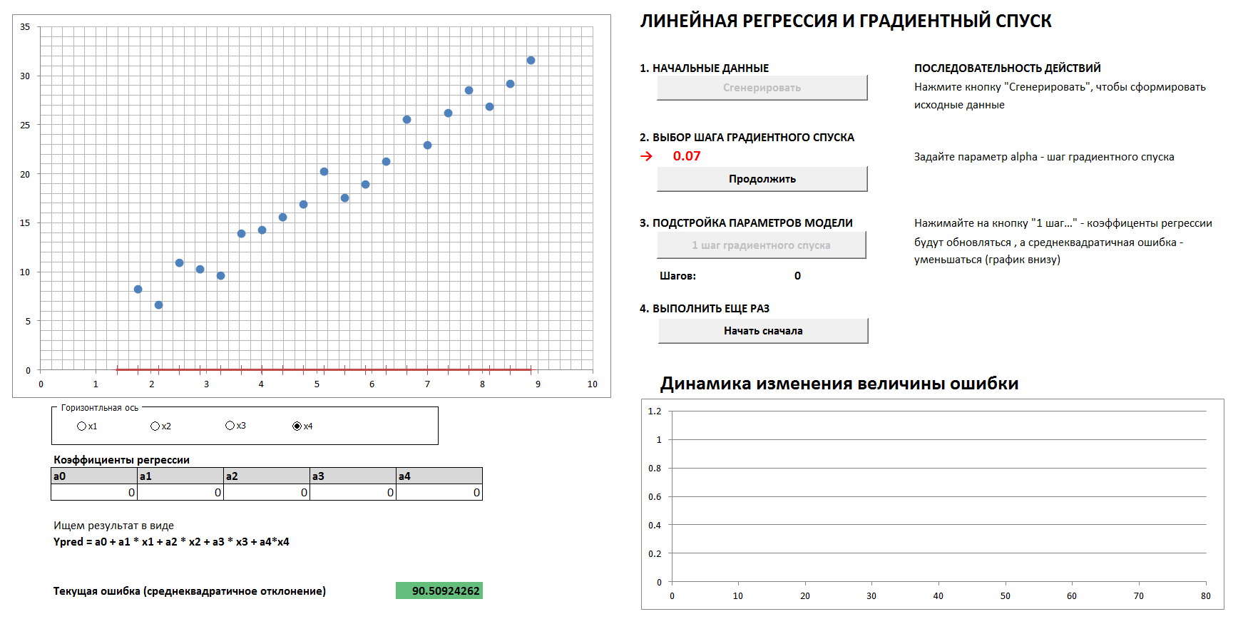
There will be a 4-dimensional case and linear regression. The linear regression coefficients will be determined in steps by the gradient descent method, initially all coefficients are zeros. A separate graph shows the dynamics of error reduction as the coefficients are more and more finely tuned. It is possible to see all four 2-dimensional projections.
If you set the gradient descent step too large, then it is clear that each time we will skip the minimum and we will arrive at the result in a larger number of steps, although in the end we will come anyway (unless we touch the descent step too much, then the algorithm will go “ in spacing "). And the graph of the dependence of the error on the iteration step will not be smooth, but “jerky”.
1. Generate data, set the gradient descent step
2. With the right choice of the gradient descent step, we smoothly and quickly enough come to the minimum

3. With the wrong choice of the gradient descent step, we skip the maximum, the error graph is “jerky”, the convergence takes a larger number of steps

and

4. With the wrong choice of the gradient descent step, we move away from minimum

(To reproduce the process with the gradient descent step values shown in the pictures, check the "reference data" box).
File - by this link, you need to enable macros, there are no viruses.
According to a respected community, is such a simplification and method of presentation acceptable? Should I translate the article into English?
To business. He wrote several application programs on MS Excel for visualization and visualization of processes that occur in different machine learning methods when analyzing data. Seeing is believing, in the end, according to the media of the culture that developed most of these methods (by the way, by no means all. The most powerful “support vector method”, or SVM, support vector machine is an invention of our compatriot Vladimir Vapnik, Moscow Institute of Management. 1963, by the way! Now he, however, teaches and works in the USA).
Three files for review
1. K-means clustering
Tasks of this kind relate to “learning without a teacher”, when we need to break down the initial data into a certain number of categories known in advance, but we don’t have any number of “correct answers”, we must extract them from the data itself. The fundamental classical problem of finding subspecies of iris flowers (Ronald Fisher, 1936!), Which is considered the first sign of this field of knowledge - is of such a nature.
The method is quite simple. We have a set of objects represented as vectors (sets of N numbers). For irises, these are sets of 4 numbers characterizing a flower: the length and width of the outer and inner perianth lobes, respectively ( Iris Fisher - Wikipedia ). As a distance, or measure of proximity between objects, the usual Cartesian metric is chosen.
Further, the centers of the clusters are selected arbitrarily (or not arbitrarily, see below), and the distances from each object to the centers of the clusters are calculated. Each object in this iteration step is marked as belonging to the nearest center. Then the center of each cluster is transferred to the arithmetic mean of the coordinates of its members (by analogy with physics it is also called the "center of mass"), and the procedure is repeated.
The process converges quickly enough. In the two-dimensional pictures, it looks like this:
1. The initial random distribution of points on the plane and the number of clusters
2. Setting the center of the clusters and assigning points to their clusters
3. Transfer of coordinates of the centers of clusters, recalculation of the points, until the centers are stabilized. The trajectory of the center of the cluster to the final position is visible.
At any time, you can set new cluster centers (without generating a new distribution of points!) And see that the partitioning process is not always unique. Mathematically, this means that for the optimized function (the sum of the squares of the distances from the points to the centers of its clusters) we find not a global, but a local minimum. This problem can be defeated either by a non-random choice of the initial centers of the clusters, or by sorting out the possible centers (sometimes it is advantageous to place them exactly at some point, then at least there is a guarantee that we will not get empty clusters). In any case, a finite set always has an exact lower bound.
You can play with this file at this link (do not forget to enable macro support. Files have been checked for viruses)
Method description on Wikipedia - k-means method
2. Approximation by polynomials and data breakdown. Retraining
A remarkable scientist and popularizer of data science K.V. Vorontsov briefly talks about machine learning methods as "the science of drawing curves through points." In this example, we will find the pattern in the data by the least squares method.
The technique of dividing the source data into “training” and “control”, as well as such a phenomenon as retraining, or “retraining” for the data is shown. With the correct approximation, we will have a certain error on the training data and a slightly larger error on the control data. If it’s wrong, it’s an exact adjustment to the training data and a huge mistake on the control.
(It is a well-known fact that through N points it is possible to draw a single curve of the N-1st degree, and this method generally does not give the desired result. The Lagrange interpolation polynomial on Wikipedia )
1. We set the initial distribution
2. Divide the points into “training” and “control” in the ratio of 70 to 30.
3. Draw an approximating curve by the training points, we see the error that it gives on the control data
4. Draw the exact curve through the training points, and we see a monstrous error on the control data (and zero on the training, but what's the point?).
Of course, the simplest variant with a single partition into “training” and “control” subsets is shown, in the general case this is done repeatedly for the best adjustment of the coefficients.
The file is available here, anti-virus checked. Turn on macros to work correctly
3. Gradient descent and error dynamics
There will be a 4-dimensional case and linear regression. The linear regression coefficients will be determined in steps by the gradient descent method, initially all coefficients are zeros. A separate graph shows the dynamics of error reduction as the coefficients are more and more finely tuned. It is possible to see all four 2-dimensional projections.
If you set the gradient descent step too large, then it is clear that each time we will skip the minimum and we will arrive at the result in a larger number of steps, although in the end we will come anyway (unless we touch the descent step too much, then the algorithm will go “ in spacing "). And the graph of the dependence of the error on the iteration step will not be smooth, but “jerky”.
1. Generate data, set the gradient descent step
2. With the right choice of the gradient descent step, we smoothly and quickly enough come to the minimum
3. With the wrong choice of the gradient descent step, we skip the maximum, the error graph is “jerky”, the convergence takes a larger number of steps
and
4. With the wrong choice of the gradient descent step, we move away from minimum
(To reproduce the process with the gradient descent step values shown in the pictures, check the "reference data" box).
File - by this link, you need to enable macros, there are no viruses.
According to a respected community, is such a simplification and method of presentation acceptable? Should I translate the article into English?