A simple explanation of path finding algorithms and A *

Part 1. General search algorithm

Introduction

Finding a path is one of those topics that are usually the most difficult for game developers. Especially poorly people understand the A * algorithm , and many think that this is some kind of incomprehensible magic.

The purpose of this article is to explain the search for the path in general and A * in particular in a very understandable and accessible way, thus putting an end to the widespread misconception that this topic is complex. With the right explanation, everything is quite simple.

Please note that in the article we will consider the search for a way for games ; unlike more academic articles, we will omit search algorithms such as Depth-First or Breadth-First. Instead, we will try to get from zero to A * as quickly as possible ..

In the first part we will explain the simplest concepts of finding a path. By understanding these basic concepts, you will realize that A * is surprisingly obvious.

Simple circuit

Although you can apply these concepts to arbitrary complex 3D environments, let's start with an extremely simple scheme: a 5 x 5 square grid. For convenience, I marked each cell with an uppercase letter.


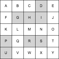
Simple mesh.

The very first thing we will do is imagine this environment as a graph. I will not explain in detail what a graph is; simply put, this is a set of circles connected by arrows. The circles are called “knots,” and the arrows are called “edges . ”

Each node represents a “state” in which the character may be. In our case, the character’s state is his position, so we create one node for each grid cell:


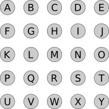
Nodes representing grid cells.

Now add the ribs. They indicate the states that can be "reached" from each given state; in our case, we can go from any cell to the next one, with the exception of blocked ones:


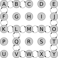
Arcs denote permissible movements between grid cells.

If we can get from A to B , then we say that B is a “neighbor” to A node.

It is worth noting that the ribs have a direction ; we need edges and from A to B , from B to A . This may seem superfluous, but not when more complex “conditions” may arise. For example, a character may fall from the roof to the floor, but is not able to jump from floor to roof. You can go from the state of "alive" to the state of "dead", but not vice versa. Etc.

Example

Let's say we want to move from A to T . We start with A . You can do exactly two things: go to the B or go to the F .

Let's say we have moved in Bed and . Now we can do two things: to return to the A or go to the C . We remember that we were already in A and considered the options there, so it makes no sense to do it again (otherwise we can spend the whole day moving A → B → A → B ...). So we go to the C .

Being in CWe have nowhere to move. Returning to B is pointless, that is, it is a dead end. Choosing the transition to B when we were in A was a bad idea; maybe you should try F instead ?

We just keep repeating this process until you find ourselves in T . At this moment, we simply recreate the path from A , returning in our steps. We are in T ; how did we get there? From o ? That is the end of the path is of the form About → T . How did we get to O ? Etc.

Please note that we are not really moving; all this was just a thought process. We continue to stand in A , and we will not move out of it until we find the whole path. When I say “moved to B ”, I mean “imagine that we moved to B ”.

General algorithm

This section is the most important part of the whole article . You absolutely must understand it in order to be able to realize the search for the way; the rest (including A * ) are just details. In this section, you will understand until you understand the meaning .

In addition, this section is incredibly simple.

Let's try to formalize our example, turning it into a pseudo-code.

We need to track the nodes that we know how to reach from the starting node. At the beginning, this is only the starting node, but in the process of “exploring” the grid, we will learn how to get to other nodes. Let's call this list of nodes reachable:

reachable = [start_node]

We also need to track the nodes already reviewed so as not to consider them again. Let's call them explored:

explored = []

Next, I will outline the core of the algorithm : at each step of the search, we select one of the nodes that we know how to reach and look at which new nodes we can get from it. If we determine how to reach the final (target) node, then the problem is solved! Otherwise, we continue the search.

So simple, what even disappoints? And this is true. But this is the whole algorithm. Let's write it down step by step with pseudo-code.

We continue to search until we either get to the final node (in this case, we find the path from the initial to the final node), or until we run out of nodes in which you can search (in this case, there is no way between the starting and ending nodes) .

while reachable is not empty:

We choose one of the nodes to which we know how to get, and which has not yet been investigated:

    node = choose_node(reachable)

If we just learned how to get to the final node, then the task is complete! We just need to build the path by following the links previousback to the start node:

    if node == goal_node:
       path = []
       while node != None:
            path.add(node)
            node = node.previous
        return path

It makes no sense to examine the node more than once, so we will track this:

    reachable.remove(node)
    explored.add(node)

We identify nodes that we cannot reach from here. We start with a list of nodes adjacent to the current one and delete the ones that we have already examined:

    new_reachable = get_adjacent_nodes(node) - explored

We take each of them:

    for adjacent in new_reachable:

If we already know how to reach the node, then ignore it. Otherwise, add it to the list reachable, tracking how it got into it:

        if adjacent not in reachable:
            adjacent.previous = node  # Remember how we got there.
            reachable.add(adjacent)

Finding the end node is one way to exit the loop. The second is when reachableit becomes empty: we have run out of nodes that can be explored, and we have not reached the final node, that is, there is no way from the initial to the final node:

return None

And that is all. This is the whole algorithm, and the path construction code is allocated in a separate method:

function find_path (start_node, end_node):
    reachable = [start_node]
    explored = []
    while reachable is not empty:
        # Choose some node we know how to reach.
        node = choose_node(reachable)
        # If we just got to the goal node, build and return the path.
        if node == goal_node:
            return build_path(goal_node)
        # Don't repeat ourselves.
        reachable.remove(node)
        explored.add(node)
        # Where can we get from here?
        new_reachable = get_adjacent_nodes(node) - explored
        for adjacent in new_reachable:
            if adjacent not in reachable
                adjacent.previous = node  # Remember how we got there.
                reachable.add(adjacent)
    # If we get here, no path was found :(
    return None

Here is a function that builds the path by following the links previousback to the start node:

function build_path (to_node):
    path = []
    while to_node != None:
        path.add(to_node)
        to_node = to_node.previous
    return path

That's all. This is the pseudocode of each path search algorithm, including A * .

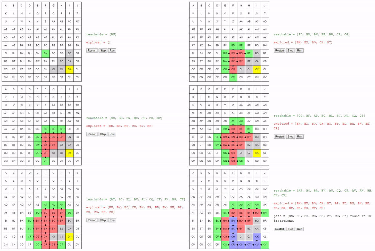
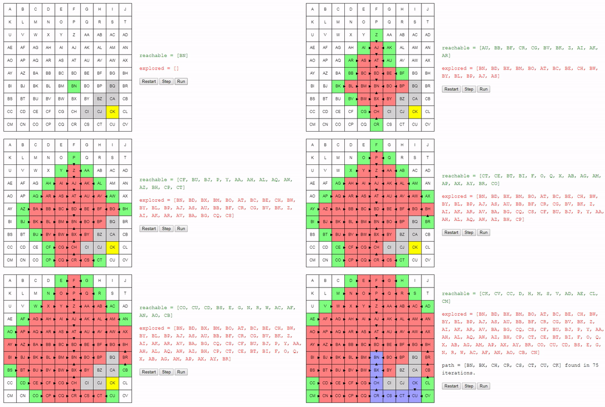
Reread this section until you understand how everything works, and, more importantly, why everything works. It would be ideal to draw an example by hand on paper, but you can also watch an interactive demo:

Interactive demo

Here is a demo and an example of the implementation of the algorithm shown above (you can run it on the page of the original article ). choose_nodejust picks a random node. You can run the algorithm step by step and look at the list of nodes reachableand explored, as well as where the links point to previous.


Notice that the search ends as soon as a path is detected; it may happen that some nodes are not even considered.

Conclusion

The algorithm presented here is a general algorithm for any path search algorithm.

But what distinguishes each algorithm from another, why A * is A * ?

Here's a tip: if you run the search in the demo several times, you will see that the algorithm does not actually always find the same path. He finds a path, and this path is not necessarily the shortest . Why?

Part 2. Search Strategies

If you do not fully understand the algorithm described in the previous section, then return to it and read it again, because it is necessary for understanding further information. When you figure it out, A * will seem completely natural and logical to you.

Secret ingredient

At the end of the previous part, I left two questions open: if each search algorithm uses the same code, why does A * behave like A * ? And why does the demo sometimes find different paths?

The answers to both questions are related to each other. Although the algorithm is well defined, I left one aspect unsolved, and as it turns out, it is the key to explaining the behavior of search algorithms:

node = choose_node(reachable)

It is this innocently looking string that distinguishes all search algorithms from each other. choose_nodeEverything depends on the implementation method .

So why does the demo find different paths? Because his method choose_nodeselects a node randomly.

Length matters

Before diving into differences in the behavior of a function choose_node, we need to fix a small oversight in the algorithm described above.

When we considered the nodes adjacent to the current, we ignored those that already know how to achieve:

if adjacent not in reachable:
    adjacent.previous = node  # Remember how we got there.
    reachable.add(adjacent)

This is a mistake: what if we just discovered the best way to get to it? In this case, you need to change the previousnode link to reflect this shorter path.

To do this, we need to know the length of the path from the starting node to any reachable node. We will call this the cost ( cost) of the path. For now, we assume that moving from a node to one of the neighboring nodes has a constant cost equal to 1.

Before starting the search, we assign a value to costeach node infinity; thanks to this, any path will be shorter than this. We will also assign costa start_nodevalue to the node 0.

Then this is how the code will look:

if adjacent not in reachable:
    reachable.add(adjacent)
# If this is a new path, or a shorter path than what we have, keep it.
if node.cost + 1 < adjacent.cost:
    adjacent.previous = node
    adjacent.cost = node.cost + 1

Same search cost

Let's look at the method now choose_node. If we strive to find the shortest possible path, then choosing a node at random is not a good idea.

It is better to choose a node that we can reach from the initial node along the shortest path; thanks to this, we generally prefer shorter paths to longer ones. This does not mean that longer paths will not be considered at all, it does mean that shorter paths will be considered first. Since the algorithm terminates immediately after finding a suitable path, this should allow us to find short paths.

Here is a possible function example choose_node:

function choose_node (reachable):
    best_node = None
    for node in reachable:
        if best_node == None or best_node.cost > node.cost:
            best_node = node
    return best_node

Intuitively, the search for this algorithm expands “radially” from the start node until it reaches the end node. Here is an interactive demo of this behavior:

Conclusion

A simple change in the method of choosing the node considered by the following allowed us to get a fairly good algorithm: it finds the shortest path from the start to the end node.

But this algorithm, to some extent, remains "stupid." He continues to search everywhere until he stumbles upon a terminal node. For example, what is the point in the example shown above to search in direction A , if it is obvious that we are moving away from the end node?

Is it possible to do choose_nodesmarter? Can we make it direct the search towards the end node , without even knowing the correct path in advance?

It turns out that we can - in the next part, we finally get tochoose_node, allowing you to turn the general path search algorithm into A * .

Part 3. Remove the veil of secrecy from A *

The algorithm obtained in the previous part is quite good: it finds the shortest path from the starting node to the final one. However, he wastes his energy: he considers the ways that a person obviously calls erroneous - they usually move away from the goal. How can this be avoided?

Magic algorithm

Imagine that we run a search algorithm on a special computer with a chip that can do magic . Thanks to this amazing chip, we can express it in a choose_nodevery simple way, which is guaranteed to create the shortest path without wasting time exploring partial paths that lead nowhere:

function choose_node (reachable):
    return magic(reachable, "любой узел, являющийся следующим на кратчайшем пути")

Sounds tempting, but magic chips still need some sort of low-level code. Here is a good approximation:

function choose_node (reachable):
    min_cost = infinity
    best_node = None
    for node in reachable:
        cost_start_to_node = node.cost
        cost_node_to_goal = magic(node, "кратчайший путь к цели")
        total_cost = cost_start_to_node + cost_node_to_goal
        if min_cost > total_cost:
            min_cost = total_cost
            best_node = node
    return best_node

This is a great way to select the next node: you select a node that gives us the shortest path from the start to the end node, which is what we need.

We also minimized the amount of magic used: we know exactly what the cost of moving from the starting node to each node is (this node.cost), and we use magic only to predict the cost of moving from the node to the final node.

Not magical, but pretty awesome A *

Unfortunately, magic chips are new, and we need support from outdated equipment. Most of the code suits us, with the exception of this line:

# Throws MuggleProcessorException
cost_node_to_goal = magic(node, "кратчайший путь к цели")

That is, we cannot use magic to find out the cost of an unexplored path. Well then, let's make a prediction. We will be optimistic and suppose that there is nothing between the current and the final nodes, and we can simply move directly:

cost_node_to_goal = distance(node, goal_node)

Note that the shortest path and the minimum distance are different: the minimum distance implies that there are absolutely no obstacles between the current and final nodes.

This estimate is quite simple to obtain. In our grid examples, this is the distance of city blocks between two nodes (i.e. abs(Ax - Bx) + abs(Ay - By)). If we could move diagonally, then the value would be equal sqrt( (Ax - Bx)^2 + (Ay - By)^2 ), and so on. Most importantly, we never get too high an estimate of value.

So here is a non-magic version choose_node:

function choose_node (reachable):
    min_cost = infinity
    best_node = None
    for node in reachable:
        cost_start_to_node = node.cost
        cost_node_to_goal = estimate_distance(node, goal_node)
        total_cost = cost_start_to_node + cost_node_to_goal
        if min_cost > total_cost:
            min_cost = total_cost
            best_node = node
    return best_node

A function that estimates the distance from the current to the final node is called a heuristic , and this search algorithm, ladies and gentlemen, is called ... A * .

Interactive demo

While you are recovering from the shock caused by the realization that the mysterious A * is actually so simple , you can look at the demo (or run it in the original article ). You will notice that, unlike the previous example, the search spends very little time moving in the wrong direction.

Conclusion

Finally, we got to the A * algorithm , which is nothing more than the general search algorithm described in the first part of the article with some improvements described in the second part and using a function choose_nodethat selects a node that, in our estimation, brings us closer to the final node. That's all.

Here's a complete pseudo-code of the main method for your reference:

function find_path (start_node, end_node):
    reachable = [start_node]
    explored = []
    while reachable is not empty:
        # Choose some node we know how to reach.
        node = choose_node(reachable)
        # If we just got to the goal node, build and return the path.
        if node == goal_node:
            return build_path(goal_node)
        # Don't repeat ourselves.
        reachable.remove(node)
        explored.add(node)
        # Where can we get from here that we haven't explored before?
        new_reachable = get_adjacent_nodes(node) - explored
        for adjacent in new_reachable:
            # First time we see this node?
            if adjacent not in reachable:
                reachable.add(adjacent)
            # If this is a new path, or a shorter path than what we have, keep it.
            if node.cost + 1 < adjacent.cost:
                adjacent.previous = node
                adjacent.cost = node.cost + 1
    # If we get here, no path was found :(
    return None

Method build_path:

function build_path (to_node):
    path = []
    while to_node != None:
        path.add(to_node)
        to_node = to_node.previous
    return path

And here is the method choose_nodethat turns it into A * :

function choose_node (reachable):
    min_cost = infinity
    best_node = None
    for node in reachable:
        cost_start_to_node = node.cost
        cost_node_to_goal = estimate_distance(node, goal_node)
        total_cost = cost_start_to_node + cost_node_to_goal
        if min_cost > total_cost:
            min_cost = total_cost
            best_node = node
    return best_node

That's all.

But why do we need part 4 ?

Now that you understand how A * works , I want to talk about some amazing areas of its application, which are far from being limited to finding paths in a grid of cells.

Part 4. A * in practice

The first three parts of the article begin with the very foundations of path search algorithms and end with a clear description of the A * algorithm . All this is great in theory, but understanding how this is applicable in practice is a completely different topic.

For example, what happens if our world is not a grid?

What if a character cannot instantly rotate 90 degrees?

How to build a graph if the world is endless?

What if we don’t care about the length of the path, but we are dependent on solar energy and we need to be under sunlight as much as possible?

How to find the shortest path to any of the two end nodes?

Cost function

In the first examples, we looked for the shortest path between the start and end nodes. However, instead of storing partial path lengths in a variable length, we named it cost. Why?

We can make A * look for not only the shortest , but also the best path, and the definition of “best” can be chosen based on our goals. When we need the shortest path, the cost is the length of the path, but if we want to minimize, for example, fuel consumption, then we need to use it as the cost. If we want to maximize the “time spent under the sun”, then the cost is the time spent without the sun. Etc.

In the general case, this means that corresponding costs are associated with each edge of the graph. In the examples shown above, the value was set implicitly and was always considered equal 1, because we considered steps along the way. But we can change the cost of the rib according to what we want to minimize.

Criterion function

Let's say our object is a car, and he needs to get to the gas station. Any refueling will suit us. It takes the shortest route to the nearest gas station.

The naive approach will be to calculate the shortest path to each refueling in turn and select the shortest one. This will work, but it will be quite a costly process.

What if we could replace one goal_nodewith a method that, according to a given node, can tell whether it is finite or not. Thanks to this, we can search for several goals at the same time. We also need to modify the heuristic so that it returns the minimum estimated cost of all possible end nodes.

Depending on the specifics of the situation, we may not be able to achieve the goal perfectly., or it will cost too much (if we send the character through half a huge map, is the difference of one inch important?), so the method is_goal_nodecan return truewhen we are "close enough".

Full certainty is not required.

Representing the world as a discrete grid may not be sufficient for many games. Take, for example, a first-person shooter or racing game. The world is discrete, but it cannot be represented as a grid.

But there is a more serious problem: what if the world is endless? In this case, even if we can present it in the form of a grid, then we simply will not be able to construct a graph corresponding to the grid, because it must be infinite.

However, not everything is lost. Of course, for the graph search algorithm, we definitely need a graph. But no one said that the graph should be comprehensive !

If you look closely at the algorithm, you will notice that we are not doing anything with the graph as a whole; we examine the graph locally, obtaining nodes that we can reach from the node in question. As can be seen from the demo A * , some nodes of the graph are not investigated at all.

So why don't we just build the graph in the research process?

We make the character’s current position the starting node. When called, get_adjacent_nodesshe can determine the possible ways in which the character is able to move from a given node, and create neighboring nodes on the fly.

Beyond Three Dimensions

Even if your world is truly a 2D mesh, there are other aspects to consider. For example, what if a character cannot instantly rotate 90 or 180 degrees, as is usually the case?

The state represented by each search node does not have to be just a position ; on the contrary, it may include an arbitrarily complex set of values. For example, if 90-degree turns take as much time as the transition from one cell to another, then the character's state can be set as [position, heading]. Each node can represent not only the character’s position, but also the direction of his gaze; and the new edges of the graph (explicit or indirect) reflect this.

If you return to the original 5x5 grid, then the initial search position can now be [A, East]. Adjacent nodes are now [B, East]and [A, South]- if we are to achieve the F , you must first adjust the direction that the path has found the form [A, East], [A, South], [F, South].

First person shooter? At least four measurements: [X, Y, Z, Heading]. Perhaps even [X, Y, Z, Heading, Health, Ammo].

Note that the more complex the state, the more complex the heuristic function should be. By itself, the A * is simple; art often arises from good heuristics.

Conclusion

The purpose of this article is to dispel the myth once and for all that A * is a mystical algorithm that cannot be deciphered. On the contrary, I showed that there is nothing mysterious in it, and in fact it can be quite simply deduced by starting from scratch.

Further reading

Amit Patel has an excellent “Introduction to the A * algorithm” [ translation on Habré] (and his other articles on various topics are also excellent!).