Developing a hexapod from scratch (part 4) - math trajectories and sequences
Hello! Hexapod development has gone one step further. This time, the trajectories of limb movement are implemented and tested - the next part of the mathematics of movement. In this article I will talk about these trajectories and basic sequences for movement. I hope it will be interesting.
Development stages:
Part 1 - design
Part 2 - assembly
Part 3 - kinematics
Part 4 - mathematics of trajectories and sequences
Part 5 - electronics
Trajectories
The essence of this mechanism is that when you set two points, you can choose the trajectory of the limb. When moving from one point to another, the coordinates will change according to certain parametric equations. The mechanism turned out to be quite powerful and allows you to get interesting curves for movement. It also implements smoothing of movements by changing the step of the parameter t - the smaller the step, the more intermediate points there will be, respectively, lower speed and higher smoothness of movement.
The procedure for setting the parameters of the trajectory in some places is a little incomprehensible and you can get confused in it. The difficulty lies in the fact that when setting the coordinates of the start and end points, the coordinates of real points in space are not always set, i.e. some coordinates set the trajectory parameters. I had to write a program that displays a given path and at the same time checks the reachability of each point of the path.
The driver supports the following motion paths:
- XYZ_LINAR is the simplest of all trajectories. The trajectory is used when moving forward, backward, up and down. All coordinates change linearly and are calculated as follows:
x = t * (x1 - x0) / 180.0f + x0;
y = t * (y1 - y0) / 180.0f + y0;
z = t * (z1 - z0) / 180.0f + z0;
Here we understand there are no problems. The coordinates specify the parallelepiped angles and they coincide with the real coordinates. The movement occurs along the diagonal of the box.Trajectory visualization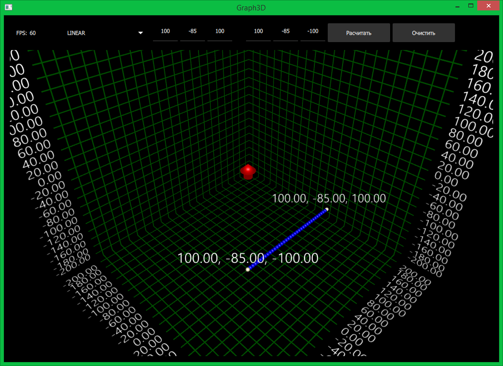

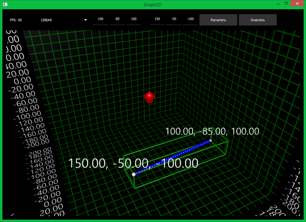
- YZ_ARC_Y_LINEAR - this trajectory allows you to implement movement along an arc. The trajectory is used when turning, when you need to move a limb on the ground. The coordinates are calculated as follows:
float R = sqrt(x0 * x0 + z0 * z0);
float atan0 = RAD_TO_DEG(atan2(x0, z0));
float atan1 = RAD_TO_DEG(atan2(x1, z1));
float t_mapped_rad = DEG_TO_RAD(t * (atan1 - atan0) / 180.0f + atan0);
x = R * sin(t_mapped_rad); // Circle Y
y = t * (y1 - y0) / 180.0f + y0;
z = R * cos(t_mapped_rad); // Circle X
This is where the fun begins. The coordinates specify the direction of the rays to limit the arc and they may not coincide with the actual coordinates. The rays are in the same plane, while the radius of the circle is equal to the length of the vector to the starting point.Trajectory visualization
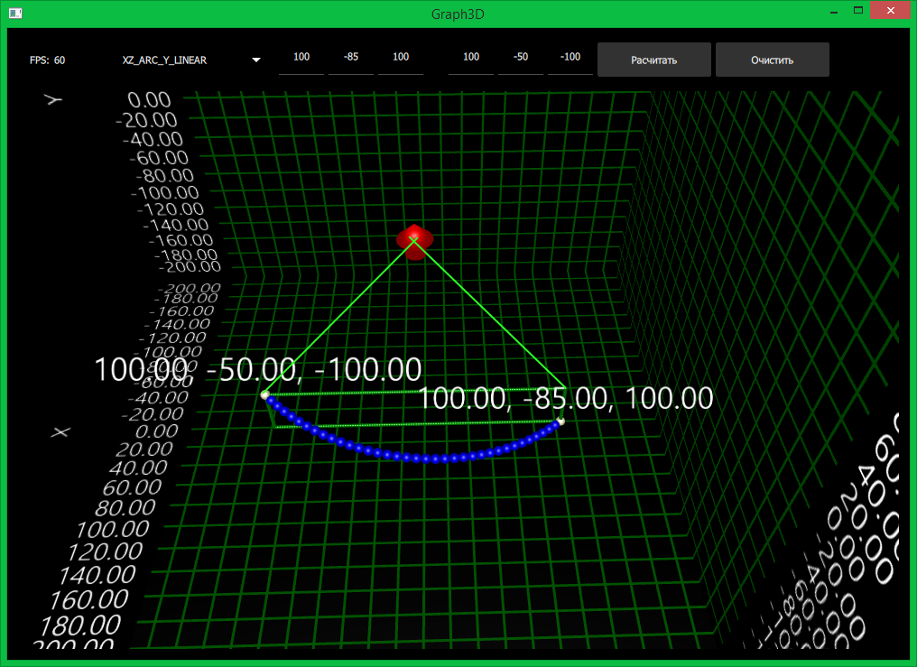
- XZ_ARC_Y_SINUS - this trajectory also allows you to implement movement along an arc, but more complex than YZ_ARC_Y_LINEAR. The trajectory is used when turning, when you need to move a limb through the air. The coordinates are calculated as follows:
float R = sqrt(x0 * x0 + z0 * z0);
float atan0 = RAD_TO_DEG(atan2(x0, z0));
float atan1 = RAD_TO_DEG(atan2(x1, z1));
float t_mapped_rad = DEG_TO_RAD(t * (atan1 - atan0) / 180.0f + atan0);
x = R * sin(t_mapped_rad); // circle Y
y = (y1 - y0) * sin(DEG_TO_RAD(t)) + y0;
z = R * cos(t_mapped_rad); // circle X
The fun continues. The coordinates also specify the direction of the rays to limit the arc, but they do NOT coincide with the actual coordinates. The Y coordinate of the target point sets the sine height.Trajectory visualization
- XZ_ELLIPTICAL_Y_SINUS - this trajectory allows you to implement movement along an ellipse. The trajectory is used when moving forward and backward, when you need to move a limb through the air. This trajectory is a complication of XZ_ARC_Y_SINUS and was needed only because of the visually ugly gait when using XZ_ARC_Y_SINUS (legs extended too much). The coordinates are calculated as follows:
float a = (z1 - z0) / 2.0f;
float b = (x1 - x0);
float c = (y1 - y0);
x = b * sin(DEG_TO_RAD(180.0f - t)) + x0; // circle Y
y = c * sin(DEG_TO_RAD(t)) + y0;
z = a * cos(DEG_TO_RAD(180.0f - t)) + z0 + a;
The coordinates specify the parallelepiped angles and they do NOT coincide with the real coordinates. The movement occurs from the lower corners of the box, located in the same plane as touching the top of its part. It’s better to look at the picture in the spoiler, I don’t know how to briefly describe it in words.Trajectory visualization
This completes the basic mathematics of the movement of the hexapod. In my project, this is a necessary minimum for the implementation of almost any movement.
Sequences
Bit of theory
Sequences are the elementary actions that make up the gait. They are divided into cyclical and non-cyclic.
- Cyclic sequences can be performed many times and at the end of each cycle should return the limbs to their original position (movement and rotation);
- Non-cyclic sequences are performed only once (ascent and descent);
Each sequence has three iteration blocks: preparation block, main block, completion block.
- Training block - contains iterations to move the limbs to the starting position for the sequence. In my case, moving forward requires putting your legs in a certain position before starting to move. It is executed once upon transition to the sequence;
- Main block - contains the main iteration of the sequence. It can be performed cyclically;
- Block completion - contains iterations for moving the limbs to the base position (the position in which the limbs are set after lifting);
The figure below shows the sequence for moving forward.
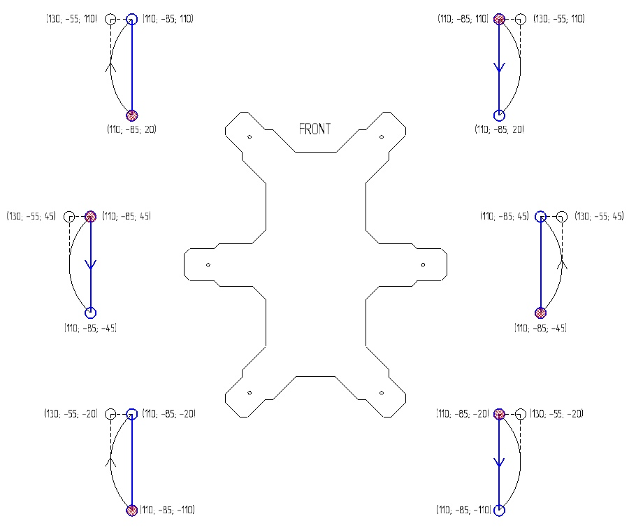
- Red dots indicate the initial position of the limbs before starting to move
- Blue lines indicate the trajectories of the limb on the ground
- The black lines indicate the trajectories of the limb in the air
- The arrows indicate the sequence
The coordinates of points are selected based on the configuration of the housing. I chose the points as close to the body as possible to reduce the length of the lever. In one cycle of the sequence, the hexapod moves by 18 cm (in 1 cycle 2 steps are taken - 1 step in 3 limbs). If you make the distance greater, then the limbs will begin to cling to each other. This parameter is limited only by the case configuration.

The sequence is defined by two points (1, 2) for each limb and two paths are used: XYZ_LINEAR (blue lines) and XZ_ELLIPTICAL_Y_SINUS (black lines). Point 1 is used by the XZ_ELLIPTICAL_Y_SINUS path to set the sine height and, accordingly, the height to which the leg will rise. Points 2 and 3 are real points that a limb reaches when moving.
The location of the points depends only on your imagination and the capabilities of the hexapod. Perhaps it all turned out a little complicated and there is a simpler option, but apparently I have not reached it yet.
Implementation
Now let’s take a look at the implementation of all this happiness. Structures with sequence parameters are as follows:
typedef struct {
    point_3d_t  point_list[SUPPORT_LIMB_COUNT];
    path_type_t path_list[SUPPORT_LIMB_COUNT];
    uint32_t    smooth_point_count;
} sequence_iteration_t;
typedef struct {
    bool is_sequence_looped;
    uint32_t main_sequence_begin;
    uint32_t finalize_sequence_begin;
    uint32_t total_iteration_count;
    sequence_iteration_t iteration_list[15];
    sequence_id_t available_sequences[SUPPORT_SEQUENCE_COUNT];
} sequence_info_t;
sequence_iteration_t - contains information about the iteration of the sequence:
- point_list - an array of points for each limb in XYZ format;
- path_list - an array of trajectories for each limb;
- smooth_point_count - sets the number of path points (parameter step t);
sequence_info_t - contains information about the entire sequence:
- is_sequence_looped - sets the type of sequence: cyclic or not;
- main_sequence_begin - sets the starting index of the main block in the iteration_list array;
- finalize_sequence_begin - sets the starting index of the completion block in the iteration_list array;
- total_iteration_count - sets the number of iterations in the sequence;
- iteration_list - an array of iterations;
- available_sequences - sets the list of sequences available for transition from the current one (for example, we cannot start walking without first getting up from the floor);
NOTE: The index of the preparation block is not intentionally indicated; it is always located at the beginning of the iteration array.
Unfortunately, I can’t provide a code for determining the sequence here, because it is quite wide and looks terrible after transfers. I just leave a link to the definition file here .
Motion processing scheme
It is worthwhile to make out all the circles of hell that the sequence goes through at run time. The processing scheme is as follows:

- MOVEMENT ENGINE - organizes processing and switching between sequences. No calculations are performed there. If simplified, then this module slips the next point to the LIBMS DRIVER module after the current processing is completed.
Module input: array of coordinates of target points.
Module output: target point for the current iteration of the sequence. - LIBMS DRIVER is the most complex of all modules. All the mathematics of movement reigns here: inverse kinematics, trajectory calculations and smoothing of movements. This module has strict synchronization with the PWM module. The calculations are carried out with a frequency of 150Hz, respectively, the control pulse to the drives is also supplied with a frequency of 150Hz.
Module input: coordinates of the target point.
Module output: servo rotation angles. - SERVO DRIVER . There is nothing special in it, except for a bunch of parameters for setting up and adjusting drives.
Module input: servo rotation angles.
Module output: control pulse width. - PWM DRIVER . PWM driver software for drive control. Here pins just twitch at the right time. The PWM synchro synchronization variable is incremented every PWM period.
Module input: control pulse width.
Module output: pulses on control pins.
I tried to make the modules independent of each other and I succeeded. This allows you to insert into this circuit any intermediate module (for example, the adaptation module to the landscape) and nothing will break at the same time, while the implementation will occur with minimal changes in the code.
Latest news and project crayfish found
Last news
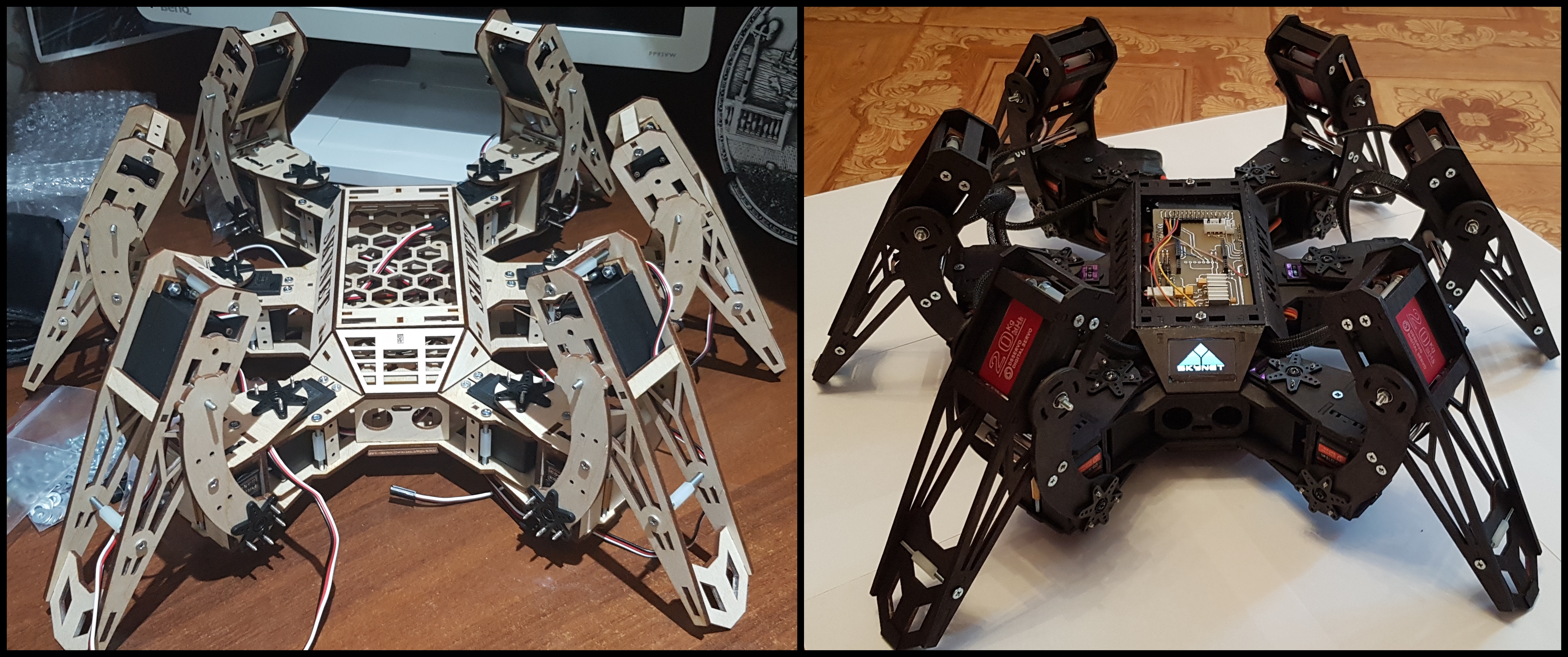
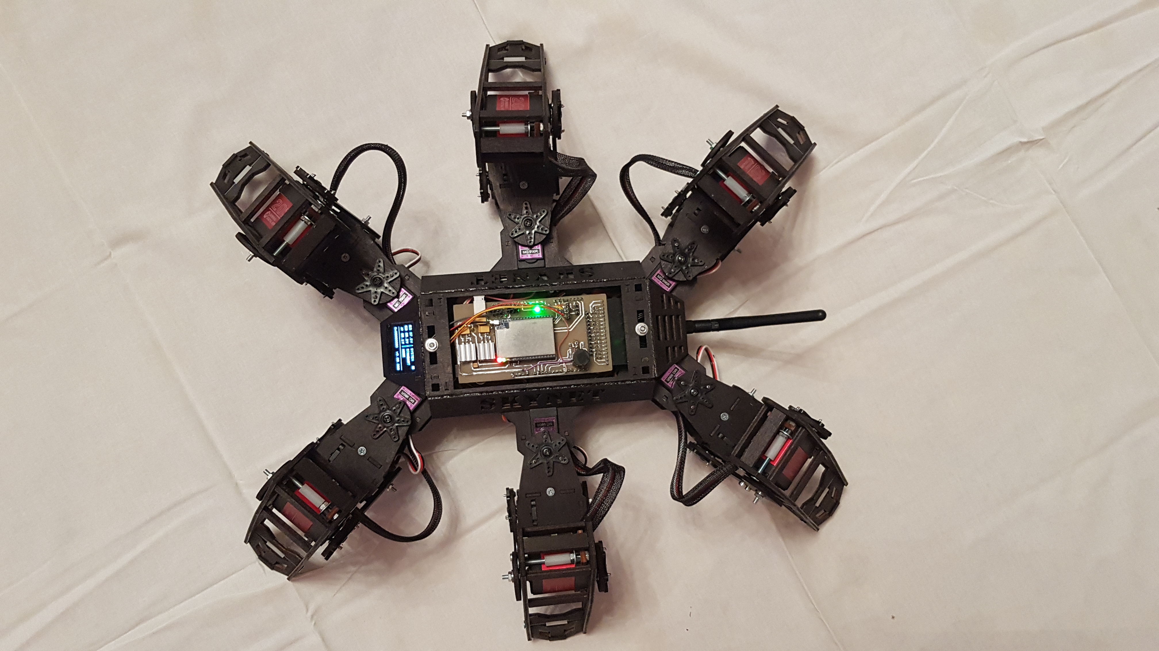
- A new test version of the case came out (archive with drawings) and I painted it a little. The complete assembly of the hexapod with the drive nozzles in the central position takes 7-8 hours of continuous assembly, and this is considering that I have already carried out this procedure more than once.Photos
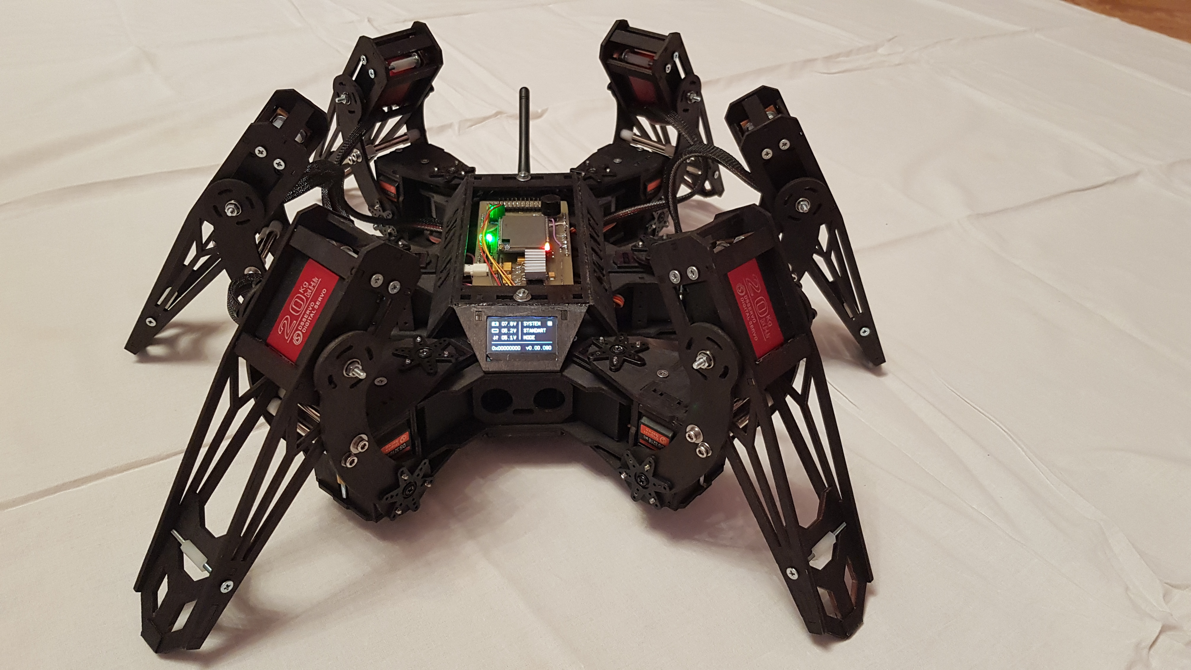

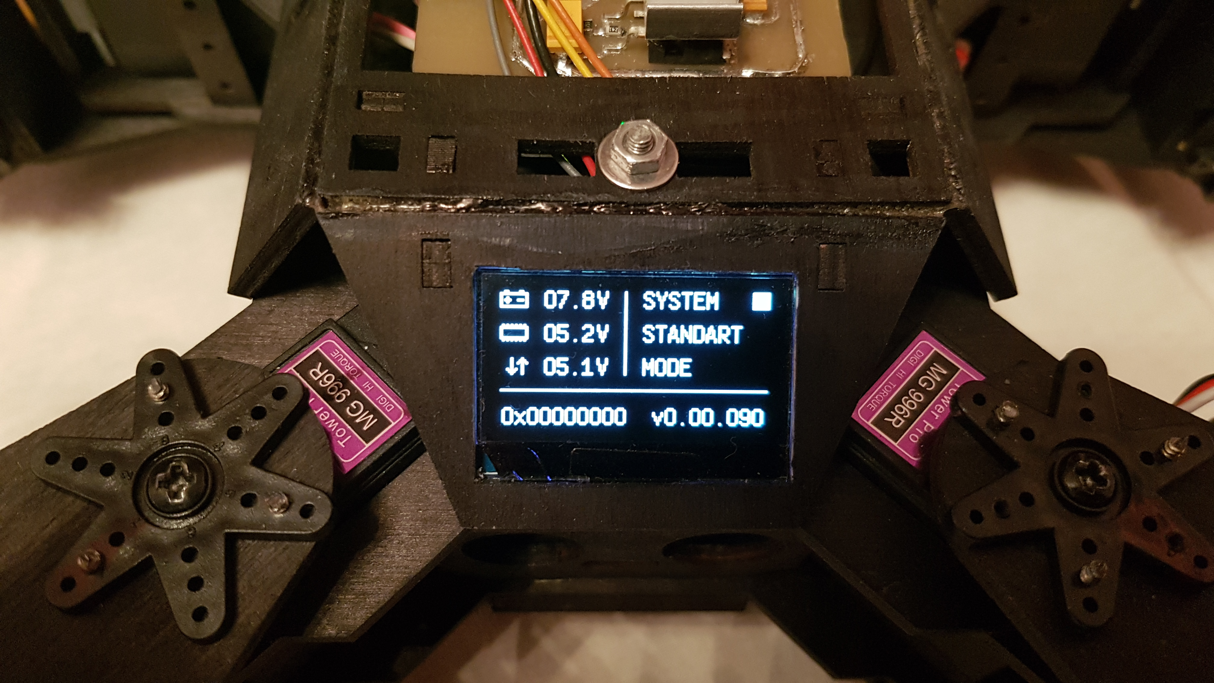
- I put an OLED display on it to display some kind of information, it turned out pretty nicely.Photos

- Started communication via WIFI. Now it is controlled from the phone (tool had to write his own)
- Reduced power supply voltage from 12V to 7V due to problems with overheating of the power board
- By the release of part 5 of the development, I will post a link to the sources, they finally acquired a state in which they are not ashamed to show people
Found crayfish
By the way, I did the calibration using this device:

- HC-SR04. I knew this sensor was bad, but I didn’t think so. In general, you need a different rangemeter
- MG996R do not meet the declared specifications. They promised 12kg \ cm - in fact 5kg \ cm at PWM with a frequency of 300Hz, at 50Hz it was even worse and besides they turned out to be analog (they promised a figure). Suitable only for turns. I had to switch to more expensive digital drives DS3218 at 20 kg / cm - in fact 23 kg / cm
- I compiled an angle-momentum table every 10 degrees and noticed that the control pulse widths for the MG996R are at different distances from each other. I had to make calibration tables for each drive and calculate the impulse individually.
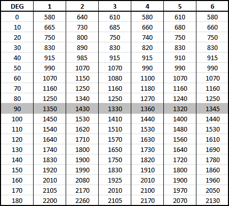
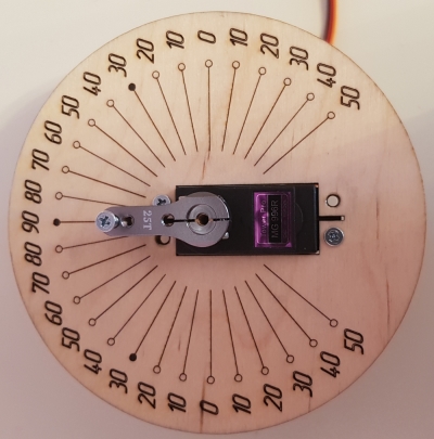
As you can see, the pulse pitch for each drive is different, it was an unexpected discovery for me. - The minimum, maximum and central values of the impulse differ due to nozzles for the drives (whatever one may say, it’s still not smooth). The figure shows the drives to which the 1500us pulse is applied and it can be seen that one nozzle is not in the center and accordingly it is necessary to adjust the pulse so that all the nozzles are in the same position.

By the way, I did the calibration using this device:
