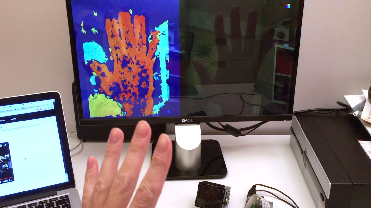
Today, all the technology of "drone building" is actively getting cheaper. Except for one: getting a map of the surrounding space. There are two extremes: either expensive lidars (thousands of dollars) and optical solutions for building a depth map (many hundreds of dollars), or quite penny solutions like ultrasonic rangefinders.
Therefore, an idea arose on the basis of an inexpensive Raspberry Pi with one camera to make a solution that would be in an empty niche and would allow you to get a depth map “for inexpensive”. And to do this in a simple programming language such as Python, so that it is available for beginners to experiment. Actually, I wanted to tell about my results. The resulting scripts with sample photos can also be run on the desktop.

Depth map from one camera.

First, a few words about the optical part. To create a depth map, two pictures are always used - from the left and right cameras. And we have raspberries with one camera. Therefore, an optical splitter was developed, which as a result gives a stereo pair to the camera.
In simple terms - if you look at the photo, then from the black box two eyes of the camera look at you. But actually the camera is one. Just a bit of optical magic.



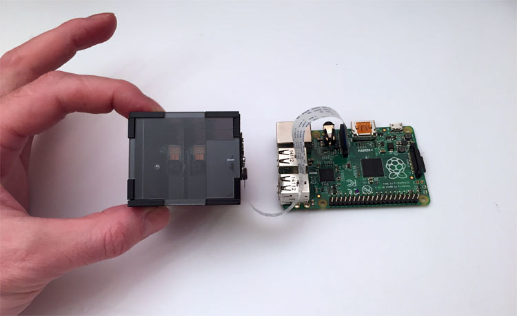
The photo shows the twelfth iteration of the device. It took a long time to get a reliable stable design, which at the same time would be inexpensive. The most difficult part is the internal mirrors, which were made to order by vacuum deposition of aluminum. If you use standard mirrors, in which the reflective layer is located under the glass, and not above it, then at the junction they form a gap that radically spoils the whole picture.

What will we work on

The raspberry image of Raspbian Wheezy was taken as the base, Python 2.7 and OpenCV 2.4 were installed, well, the required little things packages - matplotlib, numpy and others. All sorts and a link to the finished image of the card are laid out at the end of the article. Description of scripts in the form of lessons can be found on the project website

Preparing a picture for building a depth map

Since our solution is not made of metal and without ultra-precise optics, small deviations from ideal geometry are possible as a result of assembly. Plus, the camera is attached to the device with screws, so its position may not be ideal. The issue with the location of the camera is solved manually, and compensation for the "curvature" of the assembly of the structure will be done in software.

Script One - Camera Alignment

The junction of the mirrors in the picture should ideally be vertical and centered. It’s hard to do it by eye, so the first script was made. He just captures the picture from the camera in live preview mode, displays it on the screen, and in the center in overlay draws a white strip along which alignment is taking place. After the camera is correctly oriented, we tighten the cogs harder and the assembly is completed.

The second script - we get a "clean" stereo pair

Our left and right pictures are joined in the center of the image. The joint in the photo has a non-zero width - you can get rid of it only by removing the mirrors from the device, which increases the size of the structure. The raspberry’s camera has a focus set to infinity, and closely located objects (in our case, this is a junction) simply “blur”. Therefore, you just need to tell the script, which in our opinion is a “bad” zone, so that the stereo pair is cut clean into pictures. A second script was made that displays a picture and allows you to use the keys to indicate the zone to be cut.
Here's what the process looks like:

The third script - a series of photos for calibration

Basic science says that in order to successfully build a depth map, the stereo pair must be calibrated. Namely, all key points from the left picture should be at the same height and on the right picture. In this situation, the StereoBM function, which is our only real-time, can successfully do its job.
For calibration, we need to print a reference image, make a series of photos and give it to the calibration algorithm, which will calculate all the distortions and save the parameters for bringing the pictures back to normal.
So, print the “ chessboard ” and glue it on a hard flat surface. For simplicity, the serial photo was made a script with a countdown timer, which is displayed on top of the video.
Here's what a serial photography script looks like at work:





It should be especially noted that the “correctness” of the series made is critical for the calibration results. A little later we will look at the result that is obtained with incorrectly taken photographs.

Script 4 - cutting photos on stereo pairs

After a series of photos has been taken, we will make another service script that takes the entire series of photos taken and cuts it into pairs of pictures - left and right, and saves the pairs to a folder ./pairs Viewing cut pairs allows us to evaluate how well we configured the removal of defocused zones in the center of the picture. The script is quite ordinary, so I hid the video under a spoiler.

The most interesting thing is calibration, the fifth script

The calibration script feeds all stereo pairs from the ./src folder to the calibration function and plunges into thought. After his difficult work (for 15 pictures of 1280x720 on the first raspberry it takes about 5 minutes), he takes the last stereo pair, “corrects” the pictures (rectifies) and shows already corrected versions by which you can build a depth map.
Here's what the script looks like in work:

"Something went wrong"

There are times when calibration results are unexpected.
Here are a couple of striking examples:



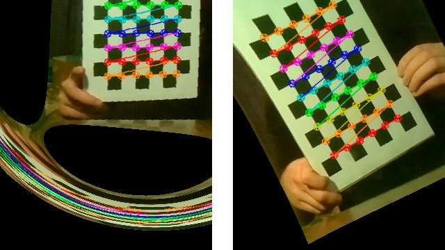
In fact, calibration is a defining moment. What we get at the stage of constructing a depth map directly depends on its quality. After a large number of experiments, the following list of shooting requirements loomed:

• The chess picture should not be parallel to the plane of the photo - always at different angles. But even without fanaticism - if you hold the board almost perpendicular to the plane of the photo, then the script simply will not find the chess in the picture.
• Light, good light. In low room lighting, and even when pulling out pictures from the video, the quality of the picture decreases. In my case, light in 90% of cases immediately corrected the situation.
• The Internet writes that the board should, if possible, occupy the maximum space in the image. Really helps.

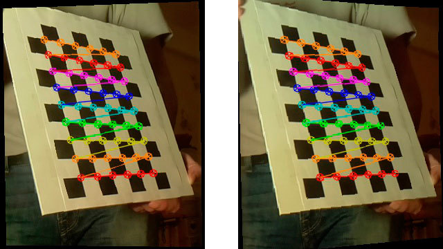
Here's what a “fixed” stereo pair looks like with good calibration results:

Script 6 - the first attempt to build a depth map

Like everything is ready - you can already build a depth map.
We load the calibration results, take a photo and boldly build a depth map using cv2.StereoBM We get something like this:



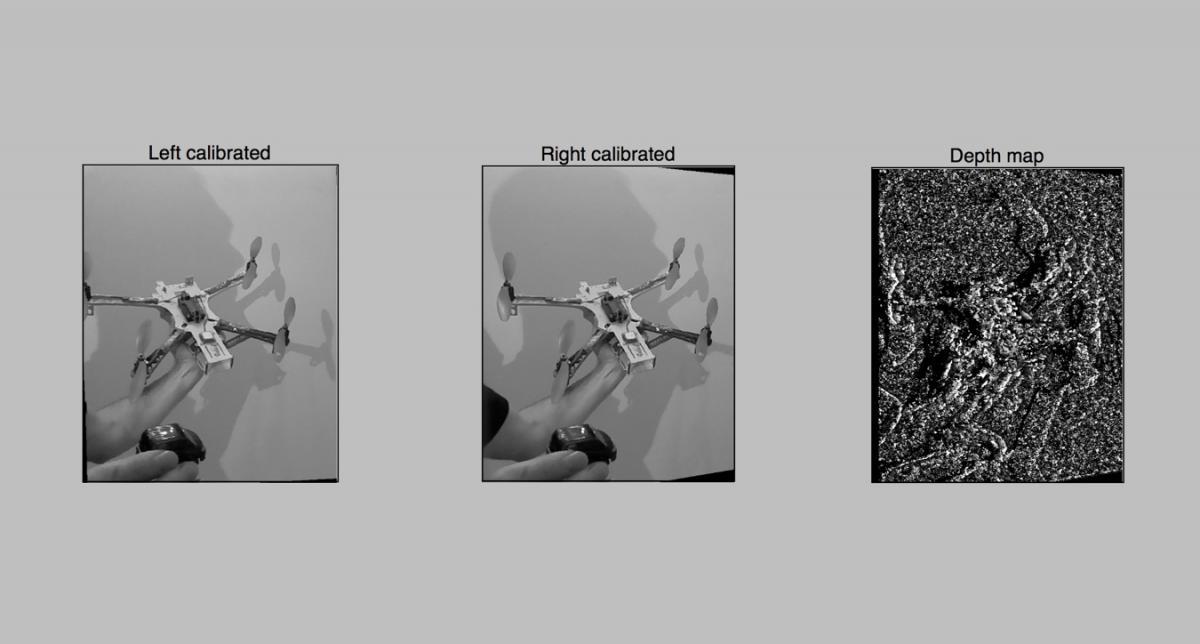
The result is not very impressive, obviously we need to tighten something. Well, let's proceed to finer tuning in the next 7th script. There we will use for construction not 2 parameters, as in StereoBM (), but almost 10, which is much more interesting.

Here are the sources of the 6th script

Script 7 - depth map with advanced settings

When the parameters are not 2 but 10, then sorting through their options with a constant restart of the scripts is wrong. Therefore, a script was made for convenient interactive tuning of the depth map. The task was not to complicate the code with the interface, so everything was done on matplotlib. The drawing of the interface in matplotlib on raspberries is quite slow, so I usually transfer the working folder from raspberries to the laptop and select the parameters there. This is how the script works:



After you have selected the parameters, the script by the Save button saves the result to the 3dmap_set.txt file in JSON format.



Practical work with the depth map showed that, first of all, you need to select the minDisparity parameter, and in conjunction with it numOfDisparities. Well, remember that numOfDisparities actually changes discretely, with step 16.
After setting up this pair, you can play with other parameters.

Features of the card settings - this is a matter of the user's taste, and depends on the task at hand. You can bring the map to a large number of small parts or display enlarged areas. For a simple avoidance of obstacles by robots, the second is more suitable. For a point cloud, the first, but performance issues come up here (we will come back to them).

What do we want to see?

Well, perhaps one of the most important points is the adjustment of the "farsightedness" of our device. When setting up the depth map, I usually place one object at a distance of about 30 cm, the second in a meter, and the rest two meters on. And when setting up the first two parameters (minDisparity and numOfDisparities) in the 7th script, I achieve the following:

• Nearest object (30 cm) - red
• Object in half a meter - yellow or green
• Objects 2-3 meters - green or light blue

As a result, we get a system configured to recognize the "near" zone of obstacles in a radius of 5-10 meters.

Working with video on the fly - script 8th, final

Well, now we have a ready-made customized system, and we would have to get a practical result. We are trying to build a depth map in real time using video from our camera, and show it in real time as it updates.

In the race for speed

So, the first measurement was done on the first Raspberry with a single-core processor.
- 4 seconds - building a map on the image of 1280x720 This is a lot.
- 2.5 seconds - on the Raspberry Pi 2, already better.
Analysis showed that only one core is used on the second raspberry. Mess! I rebuilt OpenCV using the TBB parallelization library.
- 1.5 seconds - launch on the second raspberry using multi-core. In fact, it turned out that only 2 cores are used - this still has to be tinkered with. It turned out that not only I came across this problem , so there is still room to move.
Judging by the algorithm, the speed of operation should linearly depend on the size of the processed data. Therefore, if you reduce the resolution by 2 times, then theoretically everything should work 4 times faster.
- 0.3 seconds , or about 3-4 FPS - with a half-reduced resolution of 640x360. The theory was confirmed.

Future plans

First of all, I wanted to get the most out of the multicore of the second raspberry. I’ll take a closer look at the sources of the StereoBM function and try to understand why the work is not going all the way.

The next stage promises a lot more adventure - this is using raspberry GPUs to speed up calculations.
Three possible paths are drawn here:

• There is a successful example of building a depth map using a GPU, in which it was possible to achieve 10 FPS, and it was on the first raspberry. I wrote to the author - he says that the code was written from scratch without using OpenCV, and wrote some recommendations.
• Also, an interesting approach was discovered by the Japanese friend Koichi Nakamura, who writes under the GPU in assembler under the python, here are his achievements on the github . He replied that he might try to do something for OpenCV, but not in the near future.
• Well, a request in the facebook English-speaking group of robins gave me a link to an interesting book by Jan Newmarch " Programming AudioVideo on the Raspberry Pi GPU "

If you had experience working with TBB for Raspberry OpenCV, or you were dealing with coding for raspberry GPUs, I will be grateful for additional hints . I managed to find quite a few ready-made developments for one simple reason - raspberries with two cameras are a rare occurrence. If you hook two webcams via USB, then big brakes come, and only Raspberry Pi Compute can work with two native cameras, which also needs a hefty devboard with laces and adapters.

Useful links:

Working scripts:

• Sources of all 8 scripts on github
• Card Image ( 2.6GB in the archive )

Setting up OpenCV and Python on raspberries:

• Great blog "python-OpenCV-shnik" and a manual for setting up Python and OpenCV on raspberries

StereoVision Library:

• My working fork on github
• Original by Egret on the github
• StereoVision author description on his blog

GPU work

• Lieb of the Japanese Koichi Nakamura on github - assembler for python for GPU
• Jan Newmarch Book " Programming AudioVideo on the Raspberry Pi GPU "
• If you need to work with a raspberry camera Like a Boss:
  Picamera documentation

Well, an interesting article on the habr about " To recognize images, you do not need to recognize images "