Julia and optimization
- Tutorial
The time has come to consider packages providing methods for solving optimization problems. A lot of problems can be reduced to finding a minimum of a certain function, so you should have a couple of solvers in your arsenal, and especially a whole package.
Introduction
The Julia language continues to gain popularity . At https://juliacomputing.com you can see why astronomers, robotics and financiers choose this language, and at https://academy.juliabox.com you can start free courses on learning the language and using it in every kind of engineering. For those who have seriously decided to start learning, I advise you to watch the video, read the articles and click on the jupiter laptops at https://julialang.org/learning/ or at least go through the hub from the bottom up: urgent. Now let's get to the libraries.
BlackBoxOptim
BlackBoxOptim - global optimization package for Julia ( http://julialang.org/ ). It supports both multipurpose and single-purpose optimization tasks and focuses on (meta) heuristic / stochastic algorithms (DE, NES, etc.), which DO NOT require that the function being optimized be differentiable, unlike more traditional, deterministic algorithms, which are often based on gradients / differentiability. It also supports parallel computing to speed up optimization of functions that are evaluated slowly.
Download and connect the library
]add BlackBoxOptim
using BlackBoxOptim
Set the Rosenbrock function:
f(x) = (1.0 - x[1])^2 + 100.0 * (x[2] - x[1]^2)^2We are looking for a minimum on the segment (-5; 5) for each coordinate for a two-dimensional problem:
res = bboptimize(f; SearchRange = (-5.0, 5.0), NumDimensions = 2)What the answer will be:
Starting optimization with optimizer DiffEvoOpt{FitPopulation{Float64},RadiusLimitedSelector,BlackBoxOptim.AdaptiveDiffEvoRandBin{3},RandomBound{RangePerDimSearchSpace}}
0.00 secs, 0 evals, 0 steps
Optimization stopped after 10001 steps and0.12400007247924805 seconds
Termination reason: Max number of steps (10000) reached
Steps per second = 80653.17866385692
Function evals per second = 81628.98454510146
Improvements/step = 0.2087
Total function evaluations = 10122
Best candidate found: [1.0, 1.0]
Fitness: 0.000000000
and a lot of unreadable data, but the minimum was found. Since stochastics are used, there will be a lot of function calls, so for multidimensional problems it is better to use the selection of methods
function rosenbrock(x)
  return( sum( 100*( x[2:end] - x[1:end-1].^2 ).^2 + ( x[1:end-1] - 1 ).^2 ) )
end
res = compare_optimizers(rosenbrock; SearchRange = (-5.0, 5.0), NumDimensions = 30, MaxTime = 3.0);
Convex
Convex is the Julia package for Disciplined Convex Programming (disciplinary convex programming?). Convex.jl can solve linear programs, mixed integer linear programs and DCP-compatible convex programs using various solvers, including Mosek, Gurobi, ECOS, SCS and GLPK, via the MathProgBase interface. It also supports optimization with complex variables and coefficients.
using Pkg # просто другой способ загрузки пакетов
Pkg.add("Convex")
Pkg.add("SCS")
There are many examples on the site: tomography (the process of restoring density distribution over given integrals over distribution areas. For example, you can work with tomography on black and white images), entropy maximization, logistic regression, linear programming, etc.
For example, you need to satisfy the conditions:

using Convex, SCS, LinearAlgebra
x = Variable(4)
p = satisfy(norm(x) <= 100, exp(x[1]) <= 5, x[2] >= 7, geomean(x[3], x[4]) >= x[2])
solve!(p, SCSSolver(verbose=0))
println(p.status)
x.value
Will answer
Optimal
4×1 Array{Float64,2}:
  0.08.55489232071604615.32993413315678315.329934133156783
JuMP

JuMP is a domain-specific modeling language for mathematical optimization embedded in Julia. He currently supports a number of open and commercial solvers (Artelys Knitro, BARON, Bonmin, Cbc, Clp, Couenne, CPLEX, ECOS, FICO Xpress, GLPK, Gurobi, Ipopt, MOSEK, NLopt, SCS).
JuMP makes it easy to identify and solve optimization problems without expert knowledge, but at the same time allows experts to introduce advanced algorithmic methods, such as using effective hot starts in linear programming or using callbacks to interact with branch and bound solvers. JuMP is also fast - benchmarking has shown that it can handle computations at speeds similar to specialized commercial tools such as AMPL, while maintaining the expressiveness of a universal, high-level programming language. JuMP can be easily integrated into complex workflows, including simulations and web servers.
This tool allows you to cope with such tasks as:
- LP = linear programming
- QP = quadratic programming
- SOCP = second-order conic programming (including problems with convex quadratic constraints and / or goal)
- MILP = Mixed Integer Linear Programming
- NLP = Non-linear programming
- MINLP = mixed integer nonlinear programming
- SDP = semi-definite programming
- MISDP = mixed-integer semi-defined programming
Analysis of its capabilities will be enough for several articles, so for now let's move on to the following:
Optim
Optim There are many solvers available from both free and commercial sources, and many are already wrapped for use in Julia. Few of them are written in this language. From a performance point of view, this is rarely a problem, as they are often written either in Fortran or in C. However, solvers written directly to Julia do have some advantages.
When writing Julia's software (packages), for which something needs to be optimized, the programmer can either write her own optimization procedure or use one of the many solvers available. For example, it may be something from the NLOpt set. This means adding a dependency that is not written in Julia, and more assumptions need to be made regarding the environment in which the user is located. Does the user have proper compilers? Can I use GPL code in a project?
It is also true that the use of a solver written in C or Fortran makes it impossible to use one of the main advantages of Julia: multiple dispatching. Since Optim is written entirely in Julia, we can currently use a dispatch system to simplify the use of user presets. A planned feature in this direction is to allow a user-driven choice of solvers for various stages of the algorithm, based entirely on scheduling, rather than on the predefined capabilities chosen by Optim developers.
A package on Julia also means that Optim has access to the automatic differentiation functions through packages in JuliaDiff .
Let's start:
]add Optim
using Optim
# функция Розенброка
f(x) = (1.0 - x[1])^2 + 100.0 * (x[2] - x[1]^2)^2
x0 = [0.0, 0.0]
optimize(f, x0)
We will get a response with a convenient report:
Results of Optimization Algorithm
 * Algorithm: Nelder-Mead # по умолчанию
 * Starting Point: [0.0,0.0]
 * Minimizer: [0.9999634355313174,0.9999315506115275]
 * Minimum: 3.525527e-09
 * Iterations: 60
 * Convergence: true
   *  √(Σ(yᵢ-ȳ)²)/n < 1.0e-08: true
   * Reached Maximum Number of Iterations: false
 * Objective Calls: 118
And compare with my Nelder-Mead!
My will be slower :(
using BenchmarkTools
@benchmark optimize(f, x0)
BenchmarkTools.Trial:
  memory estimate:  11.00 KiB
  allocs estimate:  419
  --------------
  minimum time:     39.078 μs (0.00% GC)
  median time:      43.420 μs (0.00% GC)
  mean time:        53.024 μs (15.02% GC)
  maximum time:     59.992 ms (99.83% GC)
  --------------
  samples:          10000
  evals/sample:     1
По ходу проверки еще и выяснилось, что моя реализация не работает, если использовать начальным приближением (0, 0). В качестве критерия остановки можно использовать объем симплекса, у меня же используется норма матрицы составленной из вершин. Здесь можно почитать про геометрическую интерпретацию нормы. В обоих случаях получается матрица из нулей — частный случай вырожденной матрицы, поэтому метод не выполняет ни одного шага. Вы можете настроить создание стартового симплекса, например, задавая удаленность его вершин от начального приближения (а не как у меня — половина длины вектора, фу, какой позор...), тогда настройка метода будет более гибкой, либо проследить, чтобы все вершины не сидели в одной точке:
for i = 1:N+1
        Xx[:,i] = fit
    end
    for i = 1:N
        Xx[i,i] += 0.5*vecl(fit) + ε
    end
Ну да, мой симплекс горааааздо медленнее:
ofNelderMid(fit = [0, 0.])
step= 1187.7234e-5 f = 2.797-18 x = [1.0, 1.0]
@benchmark ofNelderMid(fit = [0., 0.])
BenchmarkTools.Trial:
  memory estimate:  394.03 KiB
  allocs estimate:  6632
  --------------
  minimum time:     717.221 μs (0.00% GC)
  median time:      769.325 μs (0.00% GC)
  mean time:        854.644 μs (5.04% GC)
  maximum time:     50.429 ms (98.01% GC)
  --------------
  samples:          5826
  evals/sample:     1
Теперь больше резона вернуться к изучению пакета
You can choose the method used:
optimize(f, x0, LBFGS())
Results of Optimization Algorithm
 * Algorithm: L-BFGS
 * Starting Point: [0.0,0.0]
 * Minimizer: [0.9999999926662504,0.9999999853325008]
 * Minimum: 5.378388e-17
 * Iterations: 24
 * Convergence: true
   * |x - x'| ≤ 0.0e+00: false
     |x - x'| = 4.54e-11
   * |f(x) - f(x')| ≤ 0.0e+00 |f(x)|: false
     |f(x) - f(x')| = 5.30e-03 |f(x)|
   * |g(x)| ≤ 1.0e-08: true
     |g(x)| = 9.88e-14
   * Stopped by an increasing objective: false
   * Reached Maximum Number of Iterations: false
 * Objective Calls: 67
 * Gradient Calls: 67
and get detailed documentation and references to it
?LBFGS()Jacobian and Hessian functions can be specified.
function g!(G, x)
    G[1] = -2.0 * (1.0 - x[1]) - 400.0 * (x[2] - x[1]^2) * x[1]
    G[2] = 200.0 * (x[2] - x[1]^2)
end
function h!(H, x)
    H[1, 1] = 2.0 - 400.0 * x[2] + 1200.0 * x[1]^2
    H[1, 2] = -400.0 * x[1]
    H[2, 1] = -400.0 * x[1]
    H[2, 2] = 200.0
end
optimize(f, g!, h!, x0)
Results of Optimization Algorithm
 * Algorithm: Newtons Method
 * Starting Point: [0.0,0.0]
 * Minimizer: [0.9999999999999994,0.9999999999999989]
 * Minimum: 3.081488e-31
 * Iterations: 14
 * Convergence: true
   * |x - x'| ≤ 0.0e+00: false
     |x - x'| = 3.06e-09
   * |f(x) - f(x')| ≤ 0.0e+00 |f(x)|: false
     |f(x) - f(x')| = 3.03e+13 |f(x)|
   * |g(x)| ≤ 1.0e-08: true
     |g(x)| = 1.11e-15
   * Stopped by an increasing objective: false
   * Reached Maximum Number of Iterations: false
 * Objective Calls: 44
 * Gradient Calls: 44
 * Hessian Calls: 14
Apparently, automatically worked Newton's method. And this is how you can set the search area and use the gradient descent:
lower = [1.25, -2.1]
upper = [Inf, Inf]
initial_x = [2.0, 2.0]
inner_optimizer = GradientDescent()
results = optimize(f, g!, lower, upper, initial_x, Fminbox(inner_optimizer))
Results of Optimization Algorithm
 * Algorithm: Fminbox with Gradient Descent
 * Starting Point: [2.0,2.0]
 * Minimizer: [1.2500000000000002,1.5625000000000004]
 * Minimum: 6.250000e-02
 * Iterations: 8
 * Convergence: true
   * |x - x'| ≤ 0.0e+00: true
     |x - x'| = 0.00e+00
   * |f(x) - f(x')| ≤ 0.0e+00 |f(x)|: true
     |f(x) - f(x')| = 0.00e+00 |f(x)|
   * |g(x)| ≤ 1.0e-08: false
     |g(x)| = 5.00e-01
   * Stopped by an increasing objective: false
   * Reached Maximum Number of Iterations: false
 * Objective Calls: 84382
 * Gradient Calls: 84382
Well, or do not know, say, you want to solve the equation
f_univariate(x) = 2x^2+3x+1
optimize(f_univariate, -2.0, 1.0)
Results of Optimization Algorithm
 * Algorithm: Brents Method
 * Search Interval: [-2.000000, 1.000000]
 * Minimizer: -7.500000e-01
 * Minimum: -1.250000e-01
 * Iterations: 7
 * Convergence: max(|x - x_upper|, |x - x_lower|) <= 2*(1.5e-08*|x|+2.2e-16): true
 * Objective Function Calls: 8
and he picked you up the Brent Method .
Or having experimental data you need to optimize the coefficients of the model.


F(p, x) = p[1]*cos(p[2]*x) + p[2]*sin(p[1]*x)
model(p) = sum( [ (F(p, xdata[i]) - ydata[i])^2for i = 1:length(xdata)] )
xdata = [-2,-1.64,-1.33,-0.7,0,0.45,1.2,1.64,2.32,2.9]
ydata = [0.699369,0.700462,0.695354,1.03905,1.97389,2.41143,1.91091,0.919576,-0.730975,-1.42001]
res2 = optimize(model, [1.0, 0.2])
Results of Optimization Algorithm
 * Algorithm: Nelder-Mead
 * Starting Point: [1.0,0.2]
 * Minimizer: [1.8818299027162517,0.7002244825046421]
 * Minimum: 5.381270e-02
 * Iterations: 34
 * Convergence: true
   *  √(Σ(yᵢ-ȳ)²)/n < 1.0e-08: true
   * Reached Maximum Number of Iterations: false
 * Objective Calls: 71
Y = [ F(P, x) for x in xdata]
using Plots
plotly()
plot(xdata, ydata)
plot!(xdata, Y)
Bonus Creating your test function
The idea from the Habrovsky article is used . You can customize each local minimum:
"""
https://habr.com/ru/post/349660/
    :param n: количество экстремумов
    :param a: список коэффициентов крутости экстремумов, чем выше значения,
        тем быстрее функция убывает/возрастает и тем уже область экстремума
    :param c: список координат экстремумов
    :param p: список степеней гладкости в районе экстремума
    :param b: список значений функции
    :return: возвращает функцию, которой необходимо передавать одномерный список
координат точки, возвращаемая функция вернет значение тестовой функции в данной точке
"""
function feldbaum(x; n=5,
        a=[32; 43; 21; 45; .5.5],
        c=[-12; 21; -32; -2-2; 1.5-2],
        p=[96; 11; 1.51.4; 1.21.3; 0.50.5],
        b=[013.224.6])
    l = zeros(n)
    for i = 1:n
        res = 0for j = 1:size(x,1)
            res += a[i,j] * abs(x[j] - c[i,j]) ^ p[i,j]
        end
        res += b[i]
        l[i] = res
    end
    minimum(l)
end

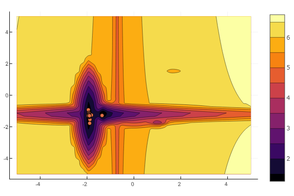
And you can give everything to the will of the almighty random
n=10
m = 2
a = rand(0:0.1:6, n, m)
c = rand(-2:0.1:2, n, m)
p = rand(0:0.1:2, n, m)
b = rand(0:0.1:8, n, m)
function feldbaum(x)
    l = zeros(n)
    for i = 1:n
        res = 0for j = 1:m
            res += a[i,j] * abs(x[j] - c[i,j]) ^ p[i,j]
        end
        res += b[i]
        l[i] = res
    end
    minimum(l)
end
But as you can see from the starting picture, you will not intimidate a swarm of particles in such a relief.
This should be finished. As you can see, Julia has a fairly powerful and modern mathematical environment that allows you to perform complex numerical studies without going down to low-level programming abstractions. And this is an excellent reason to continue learning this language.
Good luck to everyone!