Matrix Multiplication: Effective Step-by-Step Implementation

Introduction
Matrix multiplication is one of the basic algorithms that is widely used in various numerical methods, and in particular in machine learning algorithms. Many implementations of the direct and reverse signal propagation in the convolutional layers of the nerve network are based on this operation. So sometimes up to 90-95% of the total time spent on machine learning falls on this particular operation. Why it happens? The answer lies in a very effective implementation of this algorithm for processors, graphics accelerators (and, more recently, special accelerators of matrix multiplication). Matrix multiplication is one of the few algorithms that allows you to effectively use all the computing resources of modern processors and graphics accelerators. Therefore not surprising
So how is matrix multiplication algorithm implemented? Although now there are many implementations of this algorithm, including in open source. But unfortunately, the code for these implementations (mostly in assembler) is very complex. There is a good English-language article detailing these algorithms. To my surprise, I did not find analogues on Habré. As for me, this reason is quite enough to write your own article. In order to limit the scope of presentation, I limited myself to the description of a single-threaded algorithm for conventional processors. The topic of multithreading and algorithms for graphics accelerators clearly deserves a separate article.
The presentation process will be carried out in the form of steps with examples of sequential acceleration of the algorithm. I tried to write as simple as possible, but no more. I hope I succeeded ...
Statement of the problem (0th step)
In the general case, the matrix multiplication function is described as:
C[i,j] = a*C[i,j] + b*Sum(A[i,k]*B[k,j]);
Where the matrix A has size M x K, the matrix B is K x N, and the matrix C is M x N.

Without prejudice to the presentation, we can assume that a = 0 and b = 1:
C[i,j] = Sum(A[i,k]*B[k,j]);
Its implementation in C ++ “forehead” according to the formula will look as follows:
void gemm_v0(int M, int N, int K, const float * A, const float * B, float * C)
{
    for (int i = 0; i < M; ++i)
    {
        for (int j = 0; j < N; ++j)
        {
            C[i*N + j] = 0;
            for (int k = 0; k < K; ++k)
                C[i*N + j] += A[i*K + k] * B[k*N + j];
        }
    }
}
It would be foolish to expect any performance from it, and indeed test measurements show that with (M = N = K = 1152) it takes almost 1.8 seconds (test machine - i9-7900X@3.30GHz, OS - Ubuntu 04.16.6 LTS, compiler - g ++ - 6.5.0b compiler options - "-fPIC -O3 -march = haswell"). The minimum number of operations for matrix multiplication is 2 * M * N * K = 2 * 10 ^ 9. In other words, the performance is 1.6 GFLOPS, which is very far from the theoretical limit of single-threaded performance for this processor (~ 120 GFLOPS (float-32) if it is limited to using AVX2 / FMA and ~ 200 GFLOPS when using AVX-512). So what needs to be done to get closer to the theoretical limit? Further, in a series of successive optimizations, we will arrive at a solution that largely reproduces which is used in many standard libraries. In the optimization process, I will only use AVX2 / FMA, I will not touch AVX-512, since their prevalence is still small.
Eliminate obvious flaws (1st step)
First, we eliminate the most obvious shortcomings of the algorithm:
- The calculation of the addresses of the elements of arrays can be simplified by taking the constant part out of the inner loop.
- In the original version, elements of array B are not accessed sequentially. It can be ordered by changing the calculation order so that the inner loop is a sequential row traversal for all three matrices.
void gemm_v1(int M, int N, int K, const float * A, const float * B, float * C)
{
    for (int i = 0; i < M; ++i)
    {
        float * c = C + i * N;
        for (int j = 0; j < N; ++j)
            c[j] = 0;
        for (int k = 0; k < K; ++k)
        {
            const float * b = B + k * N;
            float a = A[i*K + k];
            for (int j = 0; j < N; ++j)
                c[j] += a * b[j];
        }
    }
}
The result of the test measurements shows a runtime of 250 ms, or 11.4 GFLOPS. Those. with such small edits, we got an acceleration of 8 times!
Vectorize the inner loop (2nd step)
If you carefully look at the inner loop (in the variable j), you can see that the calculations can be carried out in blocks (vectors). Almost all modern processors allow you to perform calculations on such vectors. In particular, the AVX instruction set operates on 256-bit vectors. That allows you to perform 8 operations for real numbers with single precision per cycle. AVX2 / FMA takes it one step further - it allows you to perform the combined operation of multiplication and addition (d = a * b + c) over the vector. Starting from the 4th generation, Intel desktop processors have 2 256-bit FMA modules, which allows them to theoretically perform 2 * 2 * 8 = 32 operations (float-32) per cycle. Fortunately, the AVX2 / FMA instructions are fairly easy to invoke directly from C / C ++ using the built-in functions (intrinsics). For AVX2 / FMA, they are declared in the header file.
void gemm_v2(int M, int N, int K, const float * A, const float * B, float * C)
{
    for (int i = 0; i < M; ++i)
    {
        float * c = C + i * N;
        for (int j = 0; j < N; j += 8)
            _mm256_storeu_ps(c + j + 0, _mm256_setzero_ps());
        for (int k = 0; k < K; ++k)
        {
            const float * b = B + k * N;
            __m256 a = _mm256_set1_ps(A[i*K + k]);
            for (int j = 0; j < N; j += 16)
            {
                _mm256_storeu_ps(c + j + 0, _mm256_fmadd_ps(a,
                    _mm256_loadu_ps(b + j + 0), _mm256_loadu_ps(c + j + 0)));
                _mm256_storeu_ps(c + j + 8, _mm256_fmadd_ps(a,
                    _mm256_loadu_ps(b + j + 8), _mm256_loadu_ps(c + j + 8)));
            }
        }
    }
}
Run the tests, get a time of 217 ms or 13.1 GFLOPS. Oops! Acceleration by only 15%. How so? There are two factors to consider here:
- Now smart compilers have gone (not all!), And quite cope with the task of auto-vectorization of simple loops. Already in the 1st version, the compiler actually involved the AVX2 / FMA instructions, therefore manual optimization did not give us almost any advantages.
- The calculation speed in this case does not rest on the computing capabilities of the processor, but on the speed of loading and unloading data. In this case, the processor, in order to activate 2 256-bit FMA blocks, needs to load 4 and unload 2 256-bit vectors per cycle. This is twice as much as even the bandwidth of the L1 processor cache (512/256 bit), not to mention the memory bandwidth, which is even an order of magnitude smaller (64-bit per channel)).
So, the main problem is the limited memory bandwidth in modern processors. The processor is actually idle 90% of the time, waiting for the data to load and be stored in memory.
Our further steps to optimize the algorithm will be aimed at minimizing memory access.
We write a microkernel (3rd step)
In the previous version 1 FMA operation accounts for 2 downloads and 1 upload.
Most of the downloads and unloadings occur with the resulting matrix C : the data from it must be loaded, add the product C [i] [j] + = A [i] [k] * B [k] [j] to them, and then save. And so many times. The fastest memory a processor can work with is its own registers. If we store the resulting value of the matrix C in the processor register, then in the calculation process only the value of the matrices A and B will need to be loaded . Now we have only 2 downloads per 1 FMA operation.
If we store in the registers the values of two adjacent columns of the matrix C [i] [j] and C [i] [j + 1], then we can reuse the loaded value of the matrix A [i] [k]. And for 1 FMA operation, only 1.5 downloads are required. In addition, storing the result in 2 independent registers, we will allow the processor to perform 2 FMA operations per cycle. Analogously may be stored in the registers values of the two adjacent lines - then the savings will be loaded matrix values B .

In total, Intel desktop processors starting from the 2nd generation have 16 256-bit vector registers (valid for 64-bit processor mode). 12 of them can be used to store a piece of the resulting matrix C6x16 size. As a result, we can perform 12 * 8 = 96 FMA operations by loading only 16 + 6 = 22 values from memory. And that we managed to reduce memory access from 2.0 to 0.23 downloads per 1 FMA operation - almost 10 times!
The function that calculates such a small piece of matrix C is usually called a micronucleus, the following is an example of such a function:
void micro_6x16(int K, const float * A, int lda, int step,
    const float * B, int ldb, float * C, int ldc)
{
    __m256 c00 = _mm256_setzero_ps();
    __m256 c10 = _mm256_setzero_ps();
    __m256 c20 = _mm256_setzero_ps();
    __m256 c30 = _mm256_setzero_ps();
    __m256 c40 = _mm256_setzero_ps();
    __m256 c50 = _mm256_setzero_ps();
    __m256 c01 = _mm256_setzero_ps();
    __m256 c11 = _mm256_setzero_ps();
    __m256 c21 = _mm256_setzero_ps();
    __m256 c31 = _mm256_setzero_ps();
    __m256 c41 = _mm256_setzero_ps();
    __m256 c51 = _mm256_setzero_ps();
    const int offset0 = lda * 0;
    const int offset1 = lda * 1;
    const int offset2 = lda * 2;
    const int offset3 = lda * 3;
    const int offset4 = lda * 4;
    const int offset5 = lda * 5;
    __m256 b0, b1, a0, a1;
    for (int k = 0; k < K; k++)
    {
        b0 = _mm256_loadu_ps(B + 0);
        b1 = _mm256_loadu_ps(B + 8);
        a0 = _mm256_set1_ps(A[offset0]);
        a1 = _mm256_set1_ps(A[offset1]);
        c00 = _mm256_fmadd_ps(a0, b0, c00);
        c01 = _mm256_fmadd_ps(a0, b1, c01);
        c10 = _mm256_fmadd_ps(a1, b0, c10);
        c11 = _mm256_fmadd_ps(a1, b1, c11);
        a0 = _mm256_set1_ps(A[offset2]);
        a1 = _mm256_set1_ps(A[offset3]);
        c20 = _mm256_fmadd_ps(a0, b0, c20);
        c21 = _mm256_fmadd_ps(a0, b1, c21);
        c30 = _mm256_fmadd_ps(a1, b0, c30);
        c31 = _mm256_fmadd_ps(a1, b1, c31);
        a0 = _mm256_set1_ps(A[offset4]);
        a1 = _mm256_set1_ps(A[offset5]);
        c40 = _mm256_fmadd_ps(a0, b0, c40);
        c41 = _mm256_fmadd_ps(a0, b1, c41);
        c50 = _mm256_fmadd_ps(a1, b0, c50);
        c51 = _mm256_fmadd_ps(a1, b1, c51);
        B += ldb; A += step;
    }
    _mm256_storeu_ps(C + 0, _mm256_add_ps(c00, _mm256_loadu_ps(C + 0)));
    _mm256_storeu_ps(C + 8, _mm256_add_ps(c01, _mm256_loadu_ps(C + 8)));
    C += ldc;
    _mm256_storeu_ps(C + 0, _mm256_add_ps(c10, _mm256_loadu_ps(C + 0)));
    _mm256_storeu_ps(C + 8, _mm256_add_ps(c11, _mm256_loadu_ps(C + 8)));
    C += ldc;
    _mm256_storeu_ps(C + 0, _mm256_add_ps(c20, _mm256_loadu_ps(C + 0)));
    _mm256_storeu_ps(C + 8, _mm256_add_ps(c21, _mm256_loadu_ps(C + 8)));
    C += ldc;
    _mm256_storeu_ps(C + 0, _mm256_add_ps(c30, _mm256_loadu_ps(C + 0)));
    _mm256_storeu_ps(C + 8, _mm256_add_ps(c31, _mm256_loadu_ps(C + 8)));
    C += ldc;
    _mm256_storeu_ps(C + 0, _mm256_add_ps(c40, _mm256_loadu_ps(C + 0)));
    _mm256_storeu_ps(C + 8, _mm256_add_ps(c41, _mm256_loadu_ps(C + 8)));
    C += ldc;
    _mm256_storeu_ps(C + 0, _mm256_add_ps(c50, _mm256_loadu_ps(C + 0)));
    _mm256_storeu_ps(C + 8, _mm256_add_ps(c51, _mm256_loadu_ps(C + 8)));
}
We introduce a small auxiliary function for initializing the initial value of the matrix C :
void init_c(int M, int N, float * C, int ldc)
{
    for (int i = 0; i < M; ++i, C += ldc)
        for (int j = 0; j < N; j += 8)
            _mm256_storeu_ps(C + j, _mm256_setzero_ps());
}
Here lda, ldb, ldc is the length of the line (Leading Dimension in the general case) of the corresponding matrix.
Then the multiplication function will take the following form:
void gemm_v3(int M, int N, int K, const float * A, const float * B, float * C)
{
    for (int i = 0; i < M; i += 6)
    {
        for (int j = 0; j < N; j += 16)
        {
            init_c(6, 16, C + i*N + j, N);
            micro_6x16(K, A + i*K, K, 1, B + j, N, C + i*N + j, N);
        }
    }
}
We start it and get the execution time of 78.5 ms or 36.2 GFLOPS. Those. the use of a micronucleus made it possible to accelerate matrix multiplication by almost 3 times. But the resulting speed is still far from the maximum. Where is the bottleneck now?
Reorder matrix B (4th step)
Microkernel for each iteration of the two loads 256-bit vector from the matrix Bed and .
And each time from a new line. This makes it impossible for the processor to efficiently cache this data. To correct this situation, we will make two changes:
- We copy the data of matrix B to a temporary buffer so that the data needed by one micronucleus lies nearby.
- Change the order of traversal of the matrix C : first we will go through the columns and only then through the rows. This will allow more efficient use of the matrix reordered Bed and .
To store the buffer we have a small structure:
struct buf_t
{
    float * p;
    int n;
    buf_t(int size) : n(size), p((float*)_mm_malloc(size * 4, 64)) {}
    ~buf_t() { _mm_free(p); }
};
It is worth noting here that loading and unloading of AVX vectors optimally works with aligned data, therefore special functions are used to allocate memory.
Reorder function of matrix B :
void reorder_b_16(int K, const float * B, int ldb, float * bufB)
{
    for (int k = 0; k < K; ++k, B += ldb, bufB += 16)
    {
        _mm256_storeu_ps(bufB + 0, _mm256_loadu_ps(B + 0));
        _mm256_storeu_ps(bufB + 8, _mm256_loadu_ps(B + 8));
    }
}
Well, actually the 4th version of the gemm function:
void gemm_v4(int M, int N, int K, const float * A, const float * B, float * C)
{
    for (int j = 0; j < N; j += 16)
    {
        buf_t bufB(16*K);
        reorder_b_16(K, B + j, N, bufB.p);
        for (int i = 0; i < M; i += 6)
        {
            init_c(6, 16, C + i*N + j, N);
            micro_6x16(K, A + i*K, K, 1, bufB.p, 16, C + i*N + j, N);
        }
    }
}
Test results (29.5 ms or 96.5 GFLOPS) show that we are on the right track. Actually reached about 80% of the theoretically possible maximum.
Victory? Unfortunately not. Just the size of the matrices that we used for testing (M = N = K = 1152) turned out to be convenient for this version of the algorithm. If you increase K by 100 times (M = 1152, N = 1152, K = 115200), then the efficiency of the algorithm will drop to 39.5 GFLOPS - almost 2.5 times.
We localize the data in the L1 cache (5th step)
So why does the efficiency of the algorithm decrease with increasing parameter K? The answer lies in the size of the buffer, which we used to store the values reordered Bed and . With large K values, it simply does not fit into the processor cache. The solution is to limit its size to the size of the data cache L1. For Intel processors, the L1 data cache size is 32 kb. With a buffer size limitation, the microkernel will not run over all K values, but only over the range that fits into the L1 cache. The results of intermediate calculations of matrix C will be stored in the main memory.
Let us introduce a macro core - an auxiliary function that performs calculations on the data region that interferes with the cache:
void macro_v5(int M, int N, int K, const float * A, int lda,
    const float * B, int ldb, float * bufB, float * C, int ldc)
{
    for (int j = 0; j < N; j += 16)
    {
        reorder_b_16(K, B + j, ldb, bufB);
        for (int i = 0; i < M; i += 6)
            micro_6x16(K, A + i*lda, lda, 1, bufB, 16, C + i*ldc + j, ldc);
    }
}
In the main function, we will add a cycle along K, in which we will call the macrokernel:
void gemm_v5(int M, int N, int K, const float * A, const float * B, float * C)
{
    const int L1 = 32 * 1024;
    int mK = std::min(L1 / 4 / 16, K);
    buf_t bufB(16 * mK);
    for(int k = 0; k < K; k += mK)
    {
        int dK = std::min(K, k + mK) - k;
        if(k == 0)
            init_c(M, N, C, N);
        macro_v5(M, N, dK, A + k, K, B + k*N, N, bufB.p, C, N);
    }
}
The measurement results show that we are moving in the right direction: for (M = 1152, N = 1152, K = 115200), the performance of the algorithm was 78.1 GFLOPS. This is significantly better than in the previous version, but still worse than for a medium-sized matrix.
Reorder matrix A and localize it in cache L2 (6th step)
By limiting the size K, which is processed in one pass of the microkernel, we were able to localize the data of the matrix B in the L1 cache. The data that are loaded from the matrix A is almost three times less. But let's try to localize them too, at the same time reordering the data so that they lie in sequence. Let's write a special function for this:
void reorder_a_6(const float * A, int lda, int M, int K, float * bufA)
{
    for (int i = 0; i < M; i += 6)
    {
        for (int k = 0; k < K; k += 4)
        {
            const float * pA = A + k;
            __m128 a0 = _mm_loadu_ps(pA + 0 * lda);
            __m128 a1 = _mm_loadu_ps(pA + 1 * lda);
            __m128 a2 = _mm_loadu_ps(pA + 2 * lda);
            __m128 a3 = _mm_loadu_ps(pA + 3 * lda);
            __m128 a4 = _mm_loadu_ps(pA + 4 * lda);
            __m128 a5 = _mm_loadu_ps(pA + 5 * lda);
            __m128 a00 = _mm_unpacklo_ps(a0, a2);
            __m128 a01 = _mm_unpacklo_ps(a1, a3);
            __m128 a10 = _mm_unpackhi_ps(a0, a2);
            __m128 a11 = _mm_unpackhi_ps(a1, a3);
            __m128 a20 = _mm_unpacklo_ps(a4, a5);
            __m128 a21 = _mm_unpackhi_ps(a4, a5);
            _mm_storeu_ps(bufA + 0, _mm_unpacklo_ps(a00, a01));
            _mm_storel_pi((__m64*)(bufA + 4), a20);
            _mm_storeu_ps(bufA + 6, _mm_unpackhi_ps(a00, a01));
            _mm_storeh_pi((__m64*)(bufA + 10), a20);
            _mm_storeu_ps(bufA + 12, _mm_unpacklo_ps(a10, a11));
            _mm_storel_pi((__m64*)(bufA + 16), a21);
            _mm_storeu_ps(bufA + 18, _mm_unpackhi_ps(a10, a11));
            _mm_storeh_pi((__m64*)(bufA + 22), a21);
            bufA += 24;
        }
        A += 6 * lda;
    }
}
Since, the data of matrix A now go sequentially, we no longer need the lda parameter in the macro core. The parameters of calling the microkernel have also changed:
void macro_v6(int M, int N, int K, const float * A,
    const float * B, int ldb, float * bufB, float * C, int ldc)
{
    for (int j = 0; j < N; j += 16)
    {
        reorder_b_16(K, B + j, ldb, bufB);
        for (int i = 0; i < M; i += 6)
            micro_6x16(K, A + i*K, 1, 6, bufB, 16, C + i*ldc + j, ldc);
    }
}
The buffer size for the reordered matrix A is limited by the size of the processor L2 cache (it usually ranges from 256 to 1024 kb for different types of processors). In the main function, an additional loop on the variable M is added:
void gemm_v6(int M, int N, int K, const float * A, const float * B, float * C)
{
    const int L1 = 32 * 1024, L2 = 256*1024;
    int mK = std::min(L1 / 4 / 16, K) / 4 * 4;
    int mM = std::min(L2 / 4 / mK, M) / 6 * 6;
    buf_t bufB(16 * mK);
    buf_t bufA(mK * mM);
    for(int k = 0; k < K; k += mK)
    {
        int dK = std::min(K, k + mK) - k;
        for (int i = 0; i < M; i += mM)
        {
            int dM = std::min(M, i + mM) - i;
            if (k == 0)
                init_c(dM, N, C + i * N, N);
            reorder_a_6(A + i * K + k, K, dM, dK, bufA.p);
            macro_v6(dM, N, dK, bufA.p, B + k * N, N, bufB.p, C + i * N, N);
        }
    }
}
The test results for (M = 1152, N = 1152, K = 115200) - 88.9 GFLOPS - came one step closer to the result for medium-sized matrices.
Enable the L3 cache (7th step)
In processors, in addition to the L1 and L2 cache, the L3 cache is often still available (usually its size is 1-2 MB per core). Let’s try to use it, for example, to store the reordered values of the matrices B in order to avoid unnecessary calls to the reorder_b_16 function. An additional parameter reorderB will appear in the macrokernel function, which will indicate that these matrices B are already ordered:
void macro_v7(int M, int N, int K, const float * A,
    const float * B, int ldb, float * bufB, bool reorderB, float * C, int ldc)
{
    for (int j = 0; j < N; j += 16)
    {
        if(reorderB)
            reorder_b_16(K, B + j, ldb, bufB + K*j);
        for (int i = 0; i < M; i += 6)
            micro_6x16(K, A + i*K, 1, 6, bufB + K*j, 16, C + i*ldc + j, ldc);
    }
}
In the main function, a cycle through N is added:
void gemm_v7(int M, int N, int K, const float * A, const float * B, float * C)
{
    const int L1 = 32 * 1024, L2 = 256*1024, L3 = 2*1024*1024;
    int mK = std::min(L1 / 4 / 16, K) / 4 * 4;
    int mM = std::min(L2 / 4 / mK, M) / 6 * 6;
    int mN = std::min(L3 / 4 / mK, N) / 16 * 16;
    buf_t bufB(mN * mK);
    buf_t bufA(mK * mM);
    for (int j = 0; j < N; j += mN)
    {
        int dN = std::min(N, j + mN) - j;
        for (int k = 0; k < K; k += mK)
        {
            int dK = std::min(K, k + mK) - k;
            for (int i = 0; i < M; i += mM)
            {
                int dM = std::min(M, i + mM) - i;
                if (k == 0)
                    init_c(dM, dN, C + i * N + j, N);
                reorder_a_6(A + i * K + k, K, dM, dK, bufA.p);
                macro_v7(dM, dN, dK, bufA.p, B + k * N + j, N,
                    bufB.p, i == 0, C + i * N + j, N);
            }
        }
    }
}
The measurement results for (M = 1152, N = 1152, K = 115200) give a result of 97.3 GFLOPS. Those. we even slightly exceeded the result for medium-sized matrices. In fact, we got a universal algorithm (in fact, no restrictions on the next section), which works almost equally efficiently (about 80% of the theoretically achievable maximum) for any matrix size. I propose to dwell on this and describe what we ultimately did.
General algorithm scheme
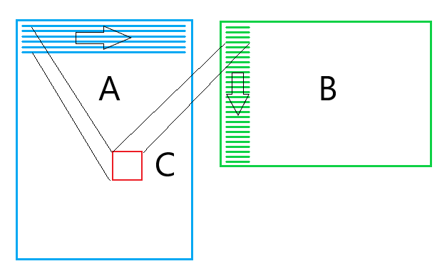
The figure below shows a diagram of the resulting algorithm:
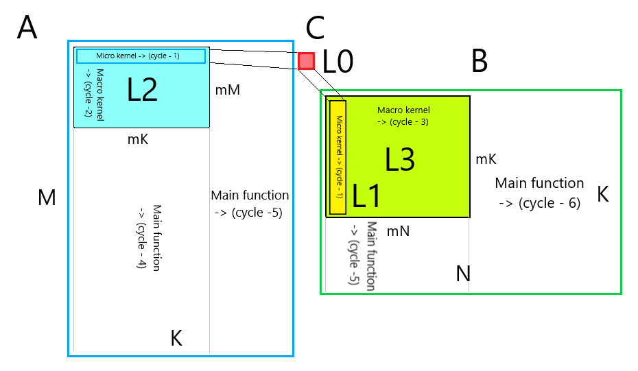
Micro core
- Cycle-1 in the variable k. The reordered data from the matrix B lies in the cache L1, the reordered data from the matrix A lies in the cache L2. The amount is accumulated in the registers (cache L0). The result is written to the main memory. The sizes of the microkernel are determined by the length of the SIMD vector and the number of vector registers. The cycle length is determined by the size of the L1 cache where B is stored .
Macro core
- Cycle 2 in variable i. It runs through the micronucleus according to the reordered data of the matrix A , which lie in the L2 cache.
- Cycle 3 in variable j. It runs through the micronucleus according to the reordered data of matrix B , which lie in the L3 cache. Optionally, reorder the missing data in Bed and .
The sizes of the macro core are determined by the size of the cache.
Main function
- Cycle 4 in variable i. Runs along the matrix A macrokernel . At each iteration reorders values A . Optionally initializes values of the matrix C .
- Cycle 5 in the variable k. Runs makroyadrom the matrices A and B .
- Cycle-6 on the variable j. Runs makroyadrom the matrix B .
What remains behind the scenes?
In the process of expounding the basic principles that are used in the matrix multiplication algorithm, I deliberately simplified the task, otherwise it would not fit into any article. Below I will describe some questions that are not important for understanding the main essence of the algorithm, but are very important for their practical implementation:
- In reality, unfortunately, the size of the matrices is not always a multiple of the sizes of the micronucleus, because the edges of the matrices have to be processed in a special way. Why do you have to implement microkernels of different sizes.
- For different types of processors, different sets of micronuclei and reordering functions are implemented. Also, there will be microkernels for double-precision numbers and for complex numbers. Fortunately, the microkernel zoo is limited only by them, and at the upper level, the code is quite universal.
- Микроядра часто пишут прямо на ассемблере. Также проводят дополнительное разворачивание циклов. Но это не приводит к существенному ускорению — основные оптимизации заключаются в эффективном использовании кэшевой иерархии памяти процессора.
- Для матриц малого размера (по любому измерению) применяют особые алгоритмы — иногда переупорядочивание не эффективно, иногда нужно применять другой порядок обхода матриц. А иногда и реализовывать особые микроядра.
- В обобщенном алгоритме матричного умножения все три матрицы могут быть транспонированы. Казалось бы число возможных алгоритмов возрастает в 8 раз! К счастью применение переупорядочивания входных данных, позволяет для всех случаев обойтись унивесальными микроядрами.
- Almost all modern processors are multi-core. And matrix multiplication libraries use multithreading to speed up computations. Usually, another 1-3 additional cycles are used for this, in which the tasks are divided into different flows.
Conclusion
The presented matrix multiplication algorithm allows you to effectively use the resources of modern processors. But it clearly shows that the maximum utilization of the resources of modern processors is far from a trivial task. The approach using micronuclei and maximum localization of data in the processor cache can be successfully used for other algorithms.
The project code with the algorithms from the article can be found on Github .
I hope you were interested!